BBBC021

MCF-7 breast cancer cells treated with 113 small molecules [Caie et al., 2010], and the standard mechanism-of-action benchmark [Ljosa et al., 2013]. bbbc021() returns the subset the benchmark annotates: 38 compounds and DMSO, 103 treatments across 12 mechanisms.

import matplotlib.pyplot as plt
import numpy as np
import pandas as pd

import mantispy as mt

adata = mt.ds.bbbc021()
adata

AnnData object with n_obs × n_vars = 632 × 473
    obs: 'Metadata_Plate', 'Metadata_Well', 'Metadata_Compound', 'Metadata_Concentration', 'Metadata_MOA', 'Metadata_CellCount', 'Metadata_SiteCount', 'Metadata_Control', 'Metadata_Perturbation'
    var: 'object', 'feature_group', 'feature', 'channel', 'scale', 'angle', 'gray_levels', 'radial_bin', 'params', 'is_feature'
    uns: 'mantispy'
    layers: None (.X)

Source

file	from	holds
ljosa_2013.csv	Cell Painting Gallery, cpg0010-caie-drugresponse/broad-az/workspace/backend	the well-level CellProfiler profiles
BBBC021_v1_image.csv	Broad Bioimage Benchmark Collection [Ljosa et al., 2012]	compound and concentration per plate and well
BBBC021_v1_moa.csv	Broad Bioimage Benchmark Collection	the mechanism per compound and concentration
632 × Image.csv	Cell Painting Gallery, workspace/analysis/<week>/<plate>/analysis/<plate>-<well>	one row per field of view, with its cell count

Every file is pinned by sha256 in the registry.

Columns mantispy adds

column	how
Metadata_Compound, Metadata_Concentration	BBBC021_v1_image.csv, joined on plate and well
Metadata_MOA	BBBC021_v1_moa.csv, joined on compound and concentration
Metadata_Control	Metadata_Compound == "DMSO"
Metadata_Perturbation	compound and concentration, "<compound>@<concentration>": what replicate wells share
Metadata_CellCount	Count_Cells of the well’s Image.csv, summed over its fields
Metadata_SiteCount	the fields of that Image.csv that contributed cells

The Image.csv files are from the same CellProfiler run as the profiles, which the profiles themselves show. CellProfiler numbers the cells of each field from 1, so a field of $n$ cells contributes object numbers $1, \dots, n$, and a well’s mean Cells_Number_Object_Number is fixed by its per-field counts $n_s$:

$$\frac{\sum_s n_s (n_s + 1) / 2}{\sum_s n_s}$$

cache = mt.settings.cache_dir / "mantispy"
profiles = pd.read_csv(cache / "ljosa_2013__analysis_batch_stable__ljosa_2013.csv").set_index(
    ["Image_Metadata_Plate", "Image_Metadata_Well"]
)["Cells_Number_Object_Number"]

checked = []
for path in sorted(cache.glob("cpg0010-caie-drugresponse/**/Image.csv")):
    n = pd.read_csv(path, usecols=["Count_Cells"])["Count_Cells"].to_numpy()
    plate, well = path.parent.name.rsplit("-", 1)
    checked.append((plate, well, (n * (n + 1) / 2).sum() / n.sum(), profiles[(plate, well)]))
checked = pd.DataFrame(checked, columns=["plate", "well", "from Image.csv", "in the profiles"])
agree = np.isclose(checked["from Image.csv"], checked["in the profiles"])
print(f"{agree.sum()} of {len(checked)} wells agree exactly")
checked.assign(difference=checked["in the profiles"] - checked["from Image.csv"])[~agree].head()

607 of 632 wells agree exactly

	plate	well	from Image.csv	in the profiles	difference
89	Week1_22401	E07	133.151679	132.958785	-0.192894
116	Week10_40115	D05	110.201258	110.444724	0.243466
124	Week10_40119	C06	31.009569	30.860577	-0.148992
143	Week2_24121	G03	41.046296	40.919505	-0.126792
145	Week2_24141	B02	96.478029	96.586436	0.108407

In the other 25 wells the two differ by at most 1.5. Those wells’ profiles averaged over nearly, but not exactly, the cells CellProfiler counted. For Week2_24121 well G03, the analysis run’s Cells.csv holds exactly the 324 cells its Image.csv counts, and their mean object number is the 41.05 the counts give, against 40.92 in the profile. Metadata_CellCount is CellProfiler’s count either way.

What it looks like

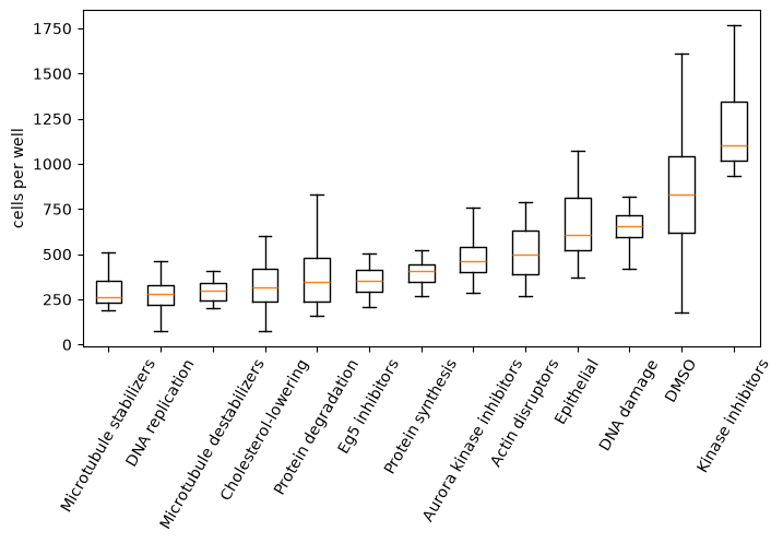
Cell count is the first thing many mechanisms change. Microtubule stabilizers and destabilizers, DNA replication inhibitors and Eg5 inhibitors all stop cells dividing, and leave a third to two fifths of the cells a DMSO well holds; the kinase inhibitors leave more than DMSO. A profile’s distance from the controls has to be read beside this, which is what cytotoxicity() does.

obs = adata.obs
order = obs.groupby("Metadata_MOA", observed=True)["Metadata_CellCount"].median().sort_values().index
fig, ax = plt.subplots(figsize=(8, 4))
ax.boxplot(
    [obs.loc[obs["Metadata_MOA"] == moa, "Metadata_CellCount"] for moa in order],
    tick_labels=list(order),
    showfliers=False,
)
ax.set_ylabel("cells per well")
ax.tick_params(axis="x", rotation=60)