4. Correcting and evaluating

Plates drift, well position matters, and cell count affects most features. This page removes those artifacts and measures whether removing them helped.

Every correction here can make results worse on a given dataset. The last section shows a real case where sphering, a standard step of the pipeline, cuts mechanism retrieval by seventy percent.

import matplotlib.pyplot as plt
import numpy as np
import scanpy as sc

import mantispy as mt

Position effects

Edge wells evaporate, corners sit at a different temperature, and dispensing drifts along a row. correct_plate_position fits Tukey’s median polish to the row and column effects of each plate and subtracts them. Median polish is used instead of a mean-based fit so that a few extreme wells do not define the gradient.

from mantispy._core.plate import well_row

cells = mt.ds.synthetic_plate(
    n_plates=2,
    n_wells=96,
    n_cells=20,
    n_features=30,
    row_gradient=3.0,
    col_gradient=2.0,
    seed=0,
)
wells = mt.tl.aggregate(cells)

rows = np.array([well_row(w) for w in wells.obs["Metadata_Well"]])
before = abs(np.corrcoef(rows, wells.X[:, 0])[0, 1])

mt.pp.correct_plate_position(wells)
after = abs(np.corrcoef(rows, wells.X[:, 0])[0, 1])
{"correlation with plate row, before": round(float(before), 3), "after": round(float(after), 3)}

{'correlation with plate row, before': 0.744, 'after': 0.016}

If treatments are laid out by column, fit the effects on the controls only, with reference="negcon", so that treatment effects are not absorbed into a column effect and subtracted.

This has a limit. A median polish can only fit a column effect for columns that contain reference rows, and most layouts put the controls in a few fixed columns, such as 1 and 2 or 23 and 24. With controls in four of twenty-four columns there is no control-only column effect to fit. Row effects still work, because controls in an edge column span every row. For column effects on a column-wise layout, the design has confounded the effect you want to correct, and the fix is a randomized layout on the next plate.

Confounders

Cell count is the most common one: a sparse well looks different from a confluent one regardless of treatment. regress_out fits each feature against the confounder within each plate and keeps the residual.

confounded = mt.ds.synthetic_plate(n_wells=96, n_cells=30, n_features=20, confounder_effect=3.0, seed=0)
profiles = mt.tl.aggregate(confounded, min_cells=0)
feature = profiles.uns["mantispy"]["truth"]["confounded_features"][0]
position = profiles.var_names.get_loc(feature)
counts = profiles.obs["Metadata_CellCount"].to_numpy(dtype=float)

before = abs(np.corrcoef(counts, profiles.X[:, position])[0, 1])
mt.pp.regress_out(profiles, keys=("Metadata_CellCount",), by=None)
after = abs(np.corrcoef(counts, profiles.X[:, position])[0, 1])
{"correlation with cell count, before": round(float(before), 3), "after": round(float(after), 3)}

{'correlation with cell count, before': 0.985, 'after': 0.0}

Missing values stay missing. Imputing them for the regression and writing the fitted value back would make an unmeasured value look like a real measurement.

Sphering

Sphering is typical variation normalization. The covariance of the negative controls describes variation that is not of interest, and whitening removes it, leaving the variation caused by the perturbations.

ZCA-cor is the default because it rotates back into the original feature basis, so the columns still match var. PCA and PCA-cor return principal components instead and warn when they overwrite X, because var then no longer describes the columns.

Sphering needs more control wells than features. With fewer, the control covariance is singular, the null directions are padded, and the transform amplifies noise. sphere warns when that happens, and the last section shows the cost.

Measuring the result

mt.metrics scores a representation with several metrics. Batch-mixing metrics and biological-signal metrics trade off against each other, and a correction that improves one at the expense of the other has not helped.

batched = mt.ds.synthetic_plate(
    n_plates=4,
    n_wells=96,
    n_cells=10,
    n_features=30,
    n_batches=2,
    batch_effect=4.0,
    n_perturbations=5,
    effect_size=3.0,
    seed=0,
)
batched = mt.tl.aggregate(batched, min_cells=0)
sc.pp.pca(batched, n_comps=15)

corrected = batched.copy()
mt.pp.normalize(corrected, method="standardize", by="Metadata_Batch")
sc.pp.pca(corrected, n_comps=15)
batched.obsm["X_batch_centred"] = corrected.obsm["X_pca"]

table = mt.metrics.evaluate_correction(
    batched,
    reps=("X_pca", "X_batch_centred"),
    label_key="Metadata_Perturbation",
    batch_key="Metadata_Batch",
)
table

	metric	representation	key	value	better
0	silhouette_label	X_pca	Metadata_Perturbation	5.682465e-01	higher
1	silhouette_batch	X_pca	Metadata_Batch	7.278925e-02	higher
2	ilisi	X_pca	Metadata_Batch	1.000000e+00	higher
3	clisi	X_pca	Metadata_Perturbation	1.009925e+00	lower
4	pc_regression	X_pca	Metadata_Batch	8.735887e-01	lower
5	silhouette_label	X_batch_centred	Metadata_Perturbation	6.665337e-01	higher
6	silhouette_batch	X_batch_centred	Metadata_Batch	9.599711e-01	higher
7	ilisi	X_batch_centred	Metadata_Batch	1.953133e+00	higher
8	clisi	X_batch_centred	Metadata_Perturbation	1.026559e+00	lower
9	pc_regression	X_batch_centred	Metadata_Batch	1.104450e-14	lower

mt.pl.metrics(table)
plt.show()

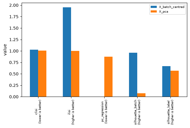
Check the better column: two of the five metrics are better when lower. pc_regression is the share of variance explained by batch, so centering each batch should lower it, and it does.

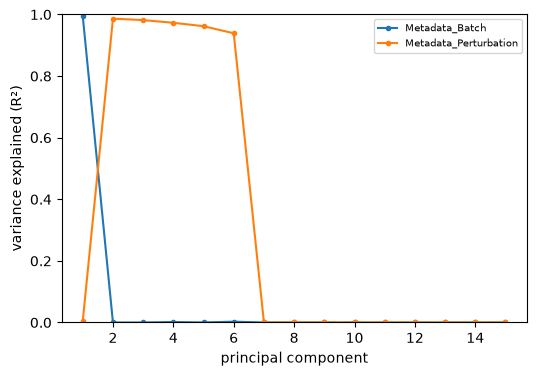
pl.batch_variance shows the same per component, which tells you where in the embedding the batch effect sits.

mt.pl.batch_variance(batched, keys=["Metadata_Batch", "Metadata_Perturbation"], use_rep="X_pca")
plt.show()

A note on Harmony

Harmony is the usual recommendation for batch correction, and mantispy wraps it as pp.harmony. It is the last step of the JUMP profiling recipe for compound and ORF profiles. It ranked in the top three in every scenario of Arevalo et al. [2024], as did Seurat RPCA. It corrects an embedding rather than the feature matrix, so run sc.pp.pca first. It needs the optional extra: pip install 'mantispy[harmony]'.

harmonypy can report convergence and return the embedding unchanged. pp.harmony compares its output with its input and warns when they are identical, since the pipeline would otherwise continue with uncorrected numbers that look plausible.

Tutorial 9 runs it on two-source JUMP data and measures the result, including a case where a batch metric disagrees with retrieval. For a correction on the features instead of an embedding, sc.pp.combat is the usual choice.

Is a perturbation doing anything?

Mean average precision (mAP) asks a retrieval question: when profiles are ranked by similarity to one profile, do its replicates rank above the profiles that should not match? It is rank-based, so it needs no correlation threshold, and its permutation null gives every group a p-value.

tl.map wraps copairs [Kalinin et al., 2025], the Broad’s implementation, so the numbers are comparable with published ones.

Compare mAP with its null, not with an intuition about scores between zero and one. Unlike accuracy, it has no fixed chance level: a random ranking’s score depends on how many positives each query has, so 0.14 can be a strong result on one screen and noise on another. null_size and the corrected_p_value column account for this.

strong = mt.ds.synthetic_plate(
    n_plates=2,
    n_wells=96,
    n_cells=20,
    n_features=40,
    n_perturbations=5,
    effect_size=4.0,
    seed=0,
)
mt.pp.normalize(strong, by="Metadata_Plate", reference="negcon")
strong = mt.tl.aggregate(strong)

mt.tl.map(strong, mode="activity", null_size=1000)
strong.uns["mantispy"]["map"][["Metadata_Perturbation", "mean_average_precision", "corrected_p_value"]]

	Metadata_Perturbation	mean_average_precision	corrected_p_value
0	pert00	1.0	0.000999
1	pert01	1.0	0.000999
2	pert02	1.0	0.000999
3	pert03	1.0	0.000999
4	pert04	1.0	0.000999

Every perturbation scores 1.0, because with an effect size of 4.0 these five are easy to retrieve. There is no DMSO row: in mode="activity" the negative controls are the reference set every treatment is scored against, so they are not scored themselves.

mode="cross_plate" asks a stricter question: replicates must retrieve each other across plates, which separates reproducible biology from a plate that happened to look uniform.

percent_replicating and grit are older readouts, kept because many published numbers use them.

A real screen: BBBC021

The sections above used synthetic data with known answers. BBBC021 is a real screen (MCF-7 cells, 38 compounds, 12 mechanisms of action), and its benchmark from Ljosa et al. [2013] is still the standard one. This downloads about 10 MB.

Degenerate features

pp.normalize flags var["degenerate_scale"]: features with no spread among the rows it was fitted on. A feature can vary across a plate and still be constant among the few control wells. mad_robustize then divides it by epsilon = 1e-18 instead of by zero, as pycytominer [Serrano et al., 2025] does, so it comes back at around 1e17 and dominates every distance computed afterwards. Feature selection does not catch it, because it measures variance across all wells.

BBBC021 has two such features. Dropping them adds eight points to the final score below.

bbbc = mt.ds.bbbc021()
bbbc

AnnData object with n_obs × n_vars = 632 × 473
    obs: 'Metadata_Plate', 'Metadata_Well', 'Metadata_Compound', 'Metadata_Concentration', 'Metadata_MOA', 'Metadata_Control', 'Metadata_Perturbation'
    var: 'object', 'feature_group', 'feature', 'channel', 'scale', 'angle', 'gray_levels', 'radial_bin', 'params', 'is_feature'
    uns: 'mantispy'
    layers: None (.X)

mt.pp.normalize(bbbc, method="mad_robustize", by="Metadata_Plate", reference="negcon")
# Two features have no spread among the DMSO wells; mad_robustize divides those by
# epsilon rather than by zero and returns them at ~1e17. See the note above.
bbbc = bbbc[:, ~bbbc.var["degenerate_scale"].to_numpy()].copy()
mt.pp.feature_select(bbbc)
bbbc = mt.pp.subset_features(bbbc)

treated = bbbc[~bbbc.obs["Metadata_Control"].to_numpy()].copy()
treated.obs["Metadata_Treatment"] = (
    treated.obs["Metadata_Compound"].astype(str) + "@" + treated.obs["Metadata_Concentration"].astype(str)
)
consensus = mt.tl.aggregate(treated, by=("Metadata_Treatment",), min_cells=0)
consensus.n_obs, consensus.obs["Metadata_MOA"].nunique()

(103, 12)

103 treatments across 12 mechanisms, the same shape as the published benchmark.

The benchmark uses the not-same-compound rule: a treatment’s nearest neighbor among treatments of a different compound should share its mechanism. Excluding the same compound prevents the task from being solved by matching a compound to itself at another dose.

def not_same_compound_accuracy(profiles):
    """Fraction of treatments whose nearest different-compound neighbour shares its MOA."""
    mt.tl.similarity(profiles, metric="cosine")
    similarity = np.asarray(profiles.obsp["similarity"]).copy()
    np.fill_diagonal(similarity, -np.inf)
    compound = profiles.obs["Metadata_Compound"].astype(str).to_numpy()
    moa = profiles.obs["Metadata_MOA"].astype(str).to_numpy()
    similarity[compound[:, None] == compound[None, :]] = -np.inf
    return float((moa[similarity.argmax(axis=1)] == moa).mean())


largest_class = consensus.obs["Metadata_MOA"].value_counts(normalize=True).iloc[0]
f"{not_same_compound_accuracy(consensus):.1%}, against {largest_class:.1%} for always guessing the largest class"

'77.7%, against 13.6% for always guessing the largest class'

Which mechanisms are resolved?

mt.tl.map(
    consensus,
    pos_sameby=["Metadata_MOA"],
    pos_diffby=["Metadata_Compound"],
    neg_diffby=["Metadata_MOA"],
    null_size=1000,
)
consensus.uns["mantispy"]["map"][["Metadata_MOA", "mean_average_precision", "below_corrected_p"]].sort_values(
    "mean_average_precision", ascending=False
)

	Metadata_MOA	mean_average_precision	below_corrected_p
11	Protein synthesis	1.000000	True
7	Kinase inhibitors	0.961905	True
1	Aurora kinase inhibitors	0.947214	True
2	Cholesterol-lowering	0.870833	True
9	Microtubule stabilizers	0.755501	True
6	Epithelial	0.741124	True
3	DNA damage	0.657428	True
4	DNA replication	0.608314	True
8	Microtubule destabilizers	0.566140	True
5	Eg5 inhibitors	0.526462	True
10	Protein degradation	0.451661	True
0	Actin disruptors	0.366134	True

Rank by the mAP column rather than the significance column. Protein synthesis, kinase and aurora kinase inhibitors separate cleanly; actin disruptors and protein degradation barely do, which matches the literature on this dataset.

below_corrected_p is True for all twelve, including the lowest. With 103 treatments the permutation null is tight enough that every mechanism differs from a random one, which does not mean it is resolved. Rank by the statistic and use the q-value only to discard, as tutorial 5 also recommends for cell-level hit calling.

Where sphering makes things worse

Sphering is a standard step in the Broad recipe, but it hurts on this dataset. The shapes show why: BBBC021 has 330 DMSO wells against 344 selected features, so the control covariance is singular.

import warnings

sphered = mt.ds.bbbc021()
mt.pp.normalize(sphered, method="mad_robustize", by="Metadata_Plate", reference="negcon")
sphered = sphered[:, ~sphered.var["degenerate_scale"].to_numpy()].copy()
mt.pp.feature_select(sphered)
sphered = mt.pp.subset_features(sphered)

with warnings.catch_warnings(record=True) as caught:
    warnings.simplefilter("always")
    mt.pp.sphere(sphered, method="ZCA-cor", reference="negcon")
print(caught[0].message)

sphering is fitted on 330 reference rows for 344 features. With fewer rows than features the covariance is singular and the transform amplifies noise (on BBBC021 it lowered not-same-compound MOA retrieval from 78% to 22%). Select fewer features first, or use more controls.

treated_sphered = sphered[~sphered.obs["Metadata_Control"].to_numpy()].copy()
treated_sphered.obs["Metadata_Treatment"] = (
    treated_sphered.obs["Metadata_Compound"].astype(str)
    + "@"
    + treated_sphered.obs["Metadata_Concentration"].astype(str)
)
consensus_sphered = mt.tl.aggregate(treated_sphered, by=("Metadata_Treatment",), min_cells=0)

{
    "without sphering": f"{not_same_compound_accuracy(consensus):.1%}",
    "with sphering": f"{not_same_compound_accuracy(consensus_sphered):.1%}",
}

{'without sphering': '77.7%', 'with sphering': '22.3%'}

Sphering cuts not-same-compound accuracy from 77.7% to 22.3%, a loss of seventy percent.

mantispy’s sphering matches pycytominer’s to seven significant figures on this data, so pycytominer shows the same drop. The method does not suit this dataset, which is why corrections should be measured with evaluate_correction instead of applied as a fixed recipe.

Run the pipeline both ways and compare. For this dataset, either select fewer features so the control matrix is well determined, or skip sphering.

The whole pipeline in eleven calls

import mantispy as mt

adata = mt.io.read_profiles("cp_output/", platemap="platemap.csv")
mt.pp.annotate_controls(adata, negcon=("DMSO",))
mt.pp.calculate_qc_metrics(adata)
mt.pp.image_qc(adata)
mt.pp.filter_images(adata)
mt.pp.filter_cells(adata)
mt.pp.normalize(adata, by="Metadata_Plate", reference="negcon")
wells = mt.tl.aggregate(adata)
mt.pp.feature_select(wells)
wells = mt.pp.subset_features(wells)
mt.tl.map(wells, mode="activity")