Reading profiles

An image-based profiling pipeline hands you a table: one row per well or per cell, a few hundred columns of CellProfiler measurements, and some metadata columns mixed in among them. read_profiles() turns one or many of those tables into an AnnData. It splits the measurements from the metadata and annotates what each feature name encodes.

import mantispy as mt

A dataset

mantispy.ds downloads whole accessions from the Cell Painting Gallery [Weisbart et al., 2024], so there is something real to read. This one is kinase inhibitors at a range of doses, eight plates of it.

adata = mt.ds.pki()
adata

AnnData object with n_obs × n_vars = 3072 × 5857
    obs: 'Metadata_plate_map_name', 'Metadata_broad_sample', 'Metadata_mg_per_ml', 'Metadata_mmoles_per_liter', 'Metadata_solvent', 'Metadata_Plate', 'Metadata_Well', 'Metadata_Site_Count', 'Metadata_Count_CellsIncludingEdges', 'Metadata_Count_Cytoplasm', 'Metadata_Count_Nuclei', 'Metadata_Count_NucleiIncludingEdges', 'Metadata_Object_Count', 'Metadata_Barcode', 'Metadata_Supplier', 'Metadata_Supplier_Catalog', 'Metadata_pert_type', 'Metadata_control_type', 'Metadata_CellCount', 'Metadata_Control', 'Metadata_Compound', 'Metadata_Concentration', 'Metadata_MOA', 'Metadata_Perturbation'
    var: 'object', 'feature_group', 'feature', 'channel', 'scale', 'angle', 'gray_levels', 'radial_bin', 'params', 'is_feature'
    uns: 'mantispy'
    layers: None (.X)

Numeric columns that parse as CellProfiler features became the feature matrix, and everything else became obs. Every metadata prefix is normalized to Metadata_, and the loader adds the columns an analysis looks for: Metadata_Compound, Metadata_Concentration, Metadata_Control and Metadata_Perturbation.

adata.obs.head()

	Metadata_plate_map_name	Metadata_broad_sample	Metadata_mg_per_ml	Metadata_mmoles_per_liter	Metadata_solvent	Metadata_Plate	Metadata_Well	Metadata_Site_Count	Metadata_Count_CellsIncludingEdges	Metadata_Count_Cytoplasm	...	Metadata_Supplier	Metadata_Supplier_Catalog	Metadata_pert_type	Metadata_control_type	Metadata_CellCount	Metadata_Control	Metadata_Compound	Metadata_Concentration	Metadata_MOA	Metadata_Perturbation
0	C-7210-01-CMP-014	NaN	NaN	NaN	DMSO	BR00122970	A01	9	1890	1758	...	NaN	DMSO	control	negcon	1758.0	True	DMSO	NaN	NaN	DMSO
1	C-7210-01-CMP-014	NaN	NaN	NaN	DMSO	BR00122970	A02	9	2137	1941	...	NaN	DMSO	control	negcon	1941.0	True	DMSO	NaN	NaN	DMSO
2	C-7210-01-CMP-014	NaN	NaN	NaN	DMSO	BR00122970	A03	9	2007	1840	...	NaN	DMSO	control	negcon	1840.0	True	DMSO	NaN	NaN	DMSO
3	C-7210-01-CMP-014	NaN	NaN	NaN	DMSO	BR00122970	A04	9	2027	1869	...	NaN	DMSO	control	negcon	1869.0	True	DMSO	NaN	NaN	DMSO
4	C-7210-01-CMP-014	NaN	NaN	NaN	DMSO	BR00122970	A05	9	2369	2165	...	NaN	DMSO	control	negcon	2165.0	True	DMSO	NaN	NaN	DMSO

5 rows × 24 columns

Plates of one screen can disagree on their columns when a channel failed on one of them, so the eight are read down to the features they share. That is on_column_mismatch="intersect"; the default is to raise instead, so a mismatch is never silent.

adata.obs.groupby("Metadata_Plate", observed=True).size()

Metadata_Plate
BR00122970    384
BR00122971    384
BR00122972    384
BR00122973    384
BR00122974    384
BR00122975    384
BR00122977    384
BR00122978    384
dtype: int64

What a feature name says

CellProfiler names a feature <object>_<feature group>_<feature>[_<channel>][_<parameters>], and read_profiles() pulls that apart into var. Correlation features measure colocalization between a pair of channels, recorded as DNA|RNA. AreaShape is geometry and carries none.

adata.var.head()

	object	feature_group	feature	channel	scale	angle	gray_levels	radial_bin	params	is_feature
Cells_AreaShape_Area	Cells	AreaShape	Area	NaN	NaN	NaN	NaN	NaN	NaN	True
Cells_AreaShape_BoundingBoxArea	Cells	AreaShape	BoundingBoxArea	NaN	NaN	NaN	NaN	NaN	NaN	True
Cells_AreaShape_BoundingBoxMaximum_X	Cells	AreaShape	BoundingBoxMaximum_X	NaN	NaN	NaN	NaN	NaN	NaN	True
Cells_AreaShape_BoundingBoxMaximum_Y	Cells	AreaShape	BoundingBoxMaximum_Y	NaN	NaN	NaN	NaN	NaN	NaN	True
Cells_AreaShape_BoundingBoxMinimum_X	Cells	AreaShape	BoundingBoxMinimum_X	NaN	NaN	NaN	NaN	NaN	NaN	True

adata.var.groupby(["object", "feature_group"], observed=True).size().sort_values(ascending=False).head(10)

object     feature_group     
Nuclei     Texture               1248
Cytoplasm  Texture               1248
Cells      Texture               1248
Nuclei     Correlation            224
Cytoplasm  Correlation            224
Cells      Correlation            224
           RadialDistribution     207
Cytoplasm  RadialDistribution     207
Cells      Granularity            128
Nuclei     Granularity            128
dtype: int64

A slice of the measurements is then a query on var instead of a regex on the names:

dna_intensity = adata[:, (adata.var["channel"] == "DNA") & (adata.var["feature_group"] == "Intensity")]
dna_intensity.shape

(3072, 45)

Reading your own files

The remaining arguments cover what has differed between datasets:

adata = mt.io.read_profiles(
    sorted(Path("profiles").glob("*/*.parquet")),
    sentinels=-999,                          # values standing for missing, replaced with NaN
    index_columns=("Metadata_Plate", "Metadata_Well"),  # joined with ":" into the observation index
    metadata_columns=("ImageNumber",),       # numeric columns that are not features
    path_columns={"Metadata_Batch": 2},      # metadata read off the file path
    on_column_mismatch="intersect",
)

path_columns maps a column name to how many directories up from the file to read the name of. That is how a batch or a plate that exists only in the directory layout gets into obs.

Pointed at a directory instead, the same call reads a CellProfiler ExportToSpreadsheet run, one row per cell with every object joined on, or the parquet parts CytoTable writes.

A first look

These are the raw measurements, and some features failed on some wells. Dropping those and scaling the rest is enough for a first look with scanpy:

import scanpy as sc

mt.pp.feature_select(adata, na_cutoff=0.0)
adata = mt.pp.subset_features(adata)
sc.pp.scale(adata)

sc.pp.pca(adata)
sc.pp.neighbors(adata)
sc.tl.umap(adata)
sc.pl.umap(adata, color=["Metadata_Plate", "Metadata_Concentration"], ncols=2)

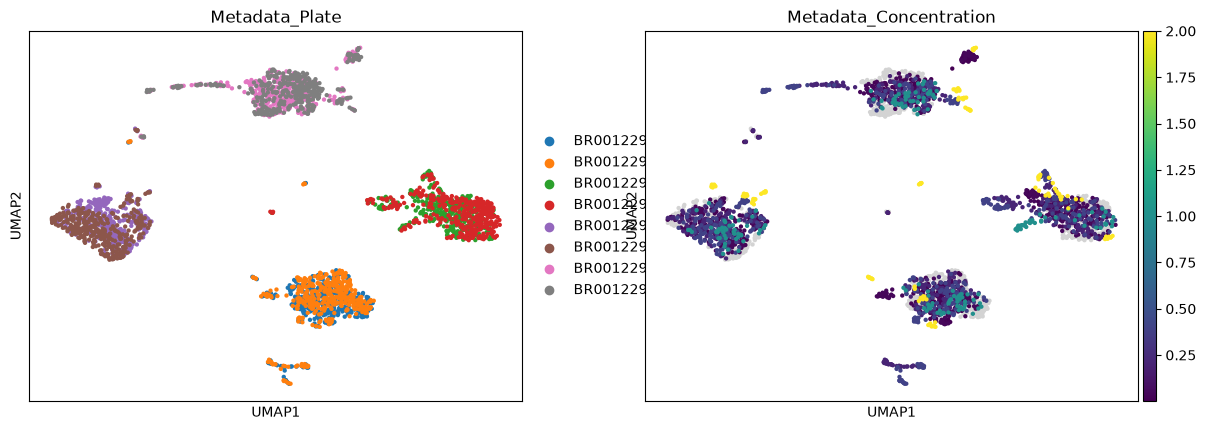
The plates separate. That is a batch effect, which a real analysis has to correct before interpreting the rest of the embedding.