0. Overview: the whole workflow on one page

mantispy does image-based profiling on AnnData. A CellProfiler run, a published profile table or a JUMP parquet goes in. Quality-controlled profiles, hit calls, effect sizes, mechanisms and enrichment come out, all stored on the object, so no result exists only in a notebook variable.

Everything here is a scverse object. adata.obs records where a profile came from, adata.var records what each feature measures (parsed from its CellProfiler name), and adata.uns["mantispy"] holds the provenance and every result table. scanpy’s PCA, neighbors, clustering and embeddings work on it unchanged, and mantispy does not reimplement them.

This page runs the workflow end to end. Each of the other tutorials covers one part of it in depth.

import matplotlib.pyplot as plt
import scanpy as sc

import mantispy as mt

The recipe

Twelve calls on BBBC021, the field’s reference benchmark. Each row links to the tutorial that covers it.

step	what it is for	page
ds.bbbc021	reading data; io.read_profiles, io.read_jump and, for images, io.read_plate are the real entry points	1
pp.normalize	put every plate on the same scale, against its own controls	2
var["degenerate_scale"]	drop features with no spread among the controls, before they dominate every distance	3
pp.feature_select	drop what is redundant or unmeasurable	3
tl.aggregate	cells to wells	2
metrics.evaluate_correction	check whether a correction helped	4
tl.hit_calling	which perturbations had an effect, with a p-value	5
tl.effect_size	which features moved, and by how much	5
tl.consensus	one signature per perturbation	5
tl.nn_moa_classify	what does this compound do	6
tl.enrich	which kinds of measurement moved	6
io.write	everything above, in one file	1

adata = mt.ds.bbbc021()

mt.pp.normalize(adata, method="mad_robustize", by="Metadata_Plate", reference="negcon")
adata = adata[:, ~adata.var["degenerate_scale"].to_numpy()].copy()
mt.pp.feature_select(adata, na_cutoff=0.0)
adata = mt.pp.subset_features(adata)

adata

AnnData object with n_obs × n_vars = 632 × 344
    obs: 'Metadata_Plate', 'Metadata_Well', 'Metadata_Compound', 'Metadata_Concentration', 'Metadata_MOA', 'Metadata_Control', 'Metadata_Perturbation'
    var: 'object', 'feature_group', 'feature', 'channel', 'scale', 'angle', 'gray_levels', 'radial_bin', 'params', 'is_feature', 'degenerate_scale', 'selected'
    uns: 'mantispy'
    layers: None (.X)

BBBC021 is distributed at well level, so there is no aggregation step here. On single cells it would be wells = mt.tl.aggregate(cells).

Is the data worth analyzing?

sc.pp.pca(adata, n_comps=30)
mt.metrics.evaluate_correction(adata, label_key="Metadata_Compound", batch_key="Metadata_Plate").round(3)

	metric	representation	key	value	better
0	silhouette_label	X_pca	Metadata_Compound	0.492	higher
1	silhouette_batch	X_pca	Metadata_Plate	0.560	higher
2	ilisi	X_pca	Metadata_Plate	10.160	higher
3	clisi	X_pca	Metadata_Compound	1.030	lower
4	pc_regression	X_pca	Metadata_Plate	0.230	lower

Hits and effects

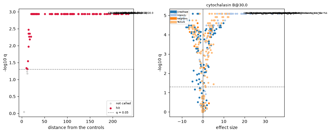
mt.tl.hit_calling(adata, groupby="Metadata_Perturbation", use_rep="X_pca", n_permutations=1000)
mt.tl.effect_size(adata, groupby="Metadata_Perturbation")

hits = adata.uns["mantispy"]["hits"]
{
    "treatments called": int(hits["is_hit"].sum()),
    "of": len(hits),
    "controls called": bool(hits.set_index("group").loc["DMSO@0.0", "is_hit"]),
}

{'treatments called': 101, 'of': 104, 'controls called': False}

fig, axes = plt.subplots(1, 2, figsize=(11, 4.5))
mt.pl.hits(adata, ax=axes[0])
mt.pl.feature_volcano(adata, group=hits.nlargest(1, "distance")["group"].iloc[0], ax=axes[1])
fig.tight_layout()
plt.show()

Mechanism

treated = adata[~adata.obs["Metadata_Control"].to_numpy()].copy()
signatures = mt.tl.consensus(treated, method="median", min_replicates=1)
signatures = signatures[signatures.obs["Metadata_MOA"].notna().to_numpy()].copy()

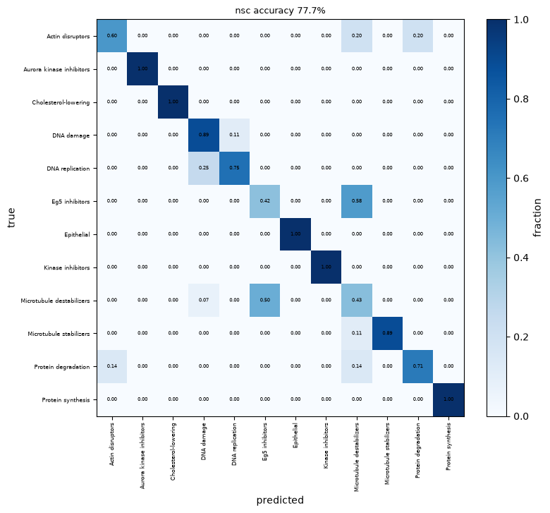
mt.tl.nn_moa_classify(signatures, scheme="nsc")
mt.tl.enrich(signatures, by="group_by_channel", method="ulm", tmin=5)
mt.tl.rank_sets(signatures, groupby="Metadata_MOA")

{
    "treatments": signatures.n_obs,
    "mechanisms": int(signatures.obs["Metadata_MOA"].nunique()),
    "not-same-compound accuracy": round(signatures.uns["mantispy"]["moa"]["accuracy"], 3),
    "chance (largest class)": round(float(signatures.obs["Metadata_MOA"].value_counts(normalize=True).iloc[0]), 3),
}

{'treatments': 103,
 'mechanisms': 12,
 'not-same-compound accuracy': 0.777,
 'chance (largest class)': 0.136}

ax = mt.pl.moa_confusion(signatures)
plt.show()

Everything is on the object

mt.io.write(signatures, "overview_signatures.h5ad")
reloaded = mt.io.read("overview_signatures.h5ad")

{
    "schema": reloaded.uns["mantispy"]["schema_version"],
    "resolution": reloaded.uns["mantispy"]["resolution"],
    "result tables": sorted(k for k in reloaded.uns["mantispy"] if k not in {"schema_version", "resolution", "params"}),
    "provenance": sorted(reloaded.uns["mantispy"]["params"]),
}

{'schema': '1.0',
 'resolution': 'perturbation',
 'result tables': ['consensus_weights', 'moa', 'moa_confusion', 'rank_sets'],
 'provenance': ['consensus', 'enrich', 'nn_moa_classify', 'rank_sets']}

Reading that file back gives the profiles, the mechanism assignments, the enrichment scores and the parameters of every step.

Where to go next

page	question
1. From CellProfiler to AnnData	how do I get my data in, and what do the feature names mean?
2. From cells to profiles	QC, normalization, aggregation
3. Trustworthy profiles	which features are worth keeping?
4. Correcting and evaluating	did my batch correction help, or hurt?
5. Hits and effects	which perturbations had an effect, and what changed?
6. Mechanism of action	what does this compound do?
7. Single-cell heterogeneity	what does a well median hide?
8. Trustworthy features and design	which features can I trust, and how many replicates do I need?
9. Scaling and laboratories	data that does not fit, and data from eleven laboratories
10. Differential features	which features moved, and are the p-values reliable?

The API reference lists every function with what it stores, the data contract and its stability guarantee, and the measured performance.