Single cells of BR00121438

The single cells behind 24 wells of one JUMP-Target-2 plate [Chandrasekaran et al., 2023], as CellProfiler measured them, at four fields of view each. The same plate’s well profiles are in JUMP-Target-2, and its images in jump_plate().

import matplotlib.pyplot as plt

import mantispy as mt

cells = mt.ds.jump_cells()
cells

AnnData object with n_obs × n_vars = 13578 × 5857
    obs: 'Metadata_ImageNumber', 'Metadata_ObjectNumber', 'Metadata_AbsPositionZ', 'Metadata_AbsTime', 'Metadata_BinningX', 'Metadata_BinningY', 'Metadata_ChannelID', 'Metadata_ChannelName', 'Metadata_Col', 'Metadata_ExposureTime', 'Metadata_FieldID', 'Metadata_ImageResolutionX', 'Metadata_ImageResolutionY', 'Metadata_ImageSizeX', 'Metadata_ImageSizeY', 'Metadata_MainEmissionWavelength', 'Metadata_MainExcitationWavelength', 'Metadata_MaxIntensity', 'Metadata_ObjectiveMagnification', 'Metadata_ObjectiveNA', 'Metadata_PlaneID', 'Metadata_Plate', 'Metadata_PositionX', 'Metadata_PositionY', 'Metadata_PositionZ', 'Metadata_Row', 'Metadata_Site', 'Metadata_Well', 'Metadata_Source', 'Metadata_JCP2022', 'Metadata_InChIKey', 'Metadata_Perturbation', 'Metadata_Control'
    var: 'object', 'feature_group', 'feature', 'channel', 'scale', 'angle', 'gray_levels', 'radial_bin', 'params', 'is_feature', 'selected'
    uns: 'mantispy'
    layers: None (.X)

Source

One ExportToSpreadsheet directory per field of view, under cpg0016-jump/source_4/workspace/analysis/2021_04_26_Batch1/BR00121438/analysis/<plate>-<well>-<site>, each with Image.csv and the Cells, Cytoplasm and Nuclei tables, about 1.5 GB in all. The JUMP annotation tables supply the perturbations, as for JUMP-Target-2.

Choices the loader makes

Which wells. Eight DMSO wells, four compounds at both of their replicate wells, and eight more compounds at one well each. The compounds that move furthest from DMSO on this plate are cytotoxic, so ranking wells by distance selects empty wells; every well here holds more than 120 cells in its first field.

wells = mt.tl.aggregate(cells, min_cells=0)
columns = ["Metadata_Well", "Metadata_Perturbation", "Metadata_Control", "Metadata_SiteCount", "Metadata_CellCount"]
wells.obs[columns].sort_values(["Metadata_Control", "Metadata_Perturbation"], ascending=[False, True])

	Metadata_Well	Metadata_Perturbation	Metadata_Control	Metadata_SiteCount	Metadata_CellCount
5	B12	JCP2022_033924	True	4	734
7	D18	JCP2022_033924	True	4	634
8	E05	JCP2022_033924	True	4	697
9	E08	JCP2022_033924	True	4	729
10	F05	JCP2022_033924	True	4	643
14	J04	JCP2022_033924	True	4	749
17	K14	JCP2022_033924	True	4	690
23	O11	JCP2022_033924	True	4	545
19	L19	JCP2022_001036	False	4	555
20	L20	JCP2022_001036	False	4	425
2	B01	JCP2022_001890	False	4	401
21	O05	JCP2022_001890	False	4	380
18	K17	JCP2022_010404	False	4	439
13	H24	JCP2022_025848	False	4	587
16	K02	JCP2022_025848	False	4	613
22	O09	JCP2022_035095	False	4	496
0	A02	JCP2022_050797	False	4	702
11	H12	JCP2022_050797	False	4	528
1	A21	JCP2022_061421	False	4	582
6	C03	JCP2022_067432	False	4	524
12	H19	JCP2022_079715	False	4	385
4	B09	JCP2022_098688	False	4	498
3	B04	JCP2022_115963	False	4	555
15	J09	JCP2022_116560	False	4	487

One row per cell. The JUMP pipeline gives Cytoplasm a parent in both Cells and Nuclei and gives Cells none, so Cytoplasm is the only object that joins all three tables, and one cytoplasm is one cell. In every field, Count_Cells in Image.csv equals the number of Cytoplasm rows.

Which features. var["selected"] marks the features feature_select() keeps after normalize() against the DMSO wells, with the features it flags as degenerate dropped first. No step of it draws a random number, so the pinned files always give the same mask. mt.ds.jump_cells(selected=True) returns only those features.

print(f"{int(cells.var['selected'].sum())} of {cells.n_vars} features selected")

1607 of 5857 features selected

Four of nine fields

The plate was imaged at nine fields per well and four are pinned here, so a well aggregated from these cells counts the cells of four fields. aggregate() records that in Metadata_SiteCount, and against the well’s count over all nine fields in JUMP-Target-2 the ratio sits near 4/9:

published = mt.ds.jump_target2(plates=["BR00121438"], annotate=False).obs.set_index("Metadata_Well")
wells.obs["all nine fields"] = published.loc[wells.obs["Metadata_Well"].astype(str), "Metadata_CellCount"].to_numpy()
wells.obs[["Metadata_Well", "Metadata_SiteCount", "Metadata_CellCount", "all nine fields"]].head()

	Metadata_Well	Metadata_SiteCount	Metadata_CellCount	all nine fields
0	A02	4	702	1527.0
1	A21	4	582	1234.0
2	B01	4	401	815.0
3	B04	4	555	1243.0
4	B09	4	498	1110.0

ratio = wells.obs["Metadata_CellCount"] / wells.obs["all nine fields"]
fig, ax = plt.subplots(figsize=(4, 4))
ax.scatter(wells.obs["all nine fields"], wells.obs["Metadata_CellCount"])
limit = wells.obs["all nine fields"].max() * 1.05
ax.plot([0, limit], [0, limit * 4 / 9], color="grey", linestyle="--", label="4/9")
ax.set_xlabel("cells in all nine fields (JUMP-Target-2)")
ax.set_ylabel("cells in the four fields here")
ax.legend()
print(f"ratio: median {ratio.median():.2f}, range {ratio.min():.2f} to {ratio.max():.2f}")

ratio: median 0.45, range 0.35 to 0.51

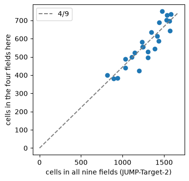
Divide by Metadata_SiteCount before comparing a count from here with one from another dataset; cytotoxicity() does so itself.