2. From cells to profiles

A screen produces millions of cells, and most analyses work on a few thousand well profiles. This page covers the steps in between: quality control at three levels, normalization against each plate’s controls, and aggregation.

The data is a synthetic plate with known ground truth, generated locally, so each result on this page can be checked against it.

import numpy as np

import mantispy as mt

adata = mt.ds.synthetic_plate(
    n_plates=2,
    n_wells=96,
    n_cells=60,
    n_features=80,
    n_images_per_well=2,
    n_bad_images=6,
    effect_size=2.0,
    nan_fraction=0.01,
    seed=0,
)
adata

AnnData object with n_obs × n_vars = 11520 × 80
    obs: 'Metadata_Plate', 'Metadata_Well', 'Metadata_Row', 'Metadata_Col', 'Metadata_Perturbation', 'Metadata_Control', 'Metadata_Batch', 'Metadata_ImageNumber', 'Metadata_CellCount'
    var: 'object', 'feature_group', 'feature', 'channel', 'scale', 'angle', 'gray_levels', 'radial_bin', 'params', 'is_feature'
    uns: 'mantispy'
    layers: None (.X)

The generator records everything it injected, and the checks below compare against that record.

truth = adata.uns["mantispy"]["truth"]
{"bad images": len(truth["bad_images"]), "perturbations affected": len(truth["affected_features"])}

{'bad images': 6, 'perturbations affected': 9}

Quality control at three levels

A cell can be bad, the image it came from can be bad, or the whole well can be. Each level has its own function. None of them delete anything. They write flags, and you decide what to drop.

Images

MeasureImageQuality gives focus, saturation and dynamic-range statistics per field of view. image_qc flags fields that are outliers within their own plate. Pooling plates would flag every field on a uniformly dimmer plate and miss a blurred field on a bright one.

mt.pp.image_qc(adata, method="mad")
result = adata.uns["mantispy"]["image_qc"]
flagged = set(result.index[~result["qc_image_pass"]])
{"flagged": sorted(flagged), "injected": sorted(truth["bad_images"])}

{'flagged': [108, 178, 200, 263, 356, 376],
 'injected': [108, 178, 200, 263, 356, 376]}

It flagged the injected images and no others. method="knn" is the alternative. Instead of asking whether any single metric is extreme, it asks whether a field’s combination of metrics is far from its neighbors, which catches images that are unusual overall without any one metric standing out.

mt.pp.filter_images(adata)
adata.shape

(11340, 80)

Cells

calculate_qc_metrics writes per-cell and per-feature statistics.

The most important one is qc_nan_fraction. Some missing values are normal in CellProfiler output, because Zernike and radial-distribution features are undefined for objects below a certain size. qc_pass therefore thresholds the fraction of missing features instead of requiring none, which would fail almost every real cell.

mt.pp.calculate_qc_metrics(adata)
{
    "cells with some missing data": float((adata.obs["qc_n_nan_features"] > 0).mean()),
    "cells passing QC": float(adata.obs["qc_pass"].mean()),
}

{'cells with some missing data': 0.5429453262786597,
 'cells passing QC': 0.9999118165784833}

mt.pp.filter_cells(adata, min_cells_per_well=20)
mt.pp.filter_features(adata, min_variance=1e-8)
adata.shape

(11339, 80)

One cell fails here: qc_pass is false for one cell of 11340, so filter_cells drops it and the plate reads 11339 rows. No feature is constant, so filter_features keeps all 80 columns. On a plate where cells or features fail in numbers, the filters remove much more.

Wells

well_qc summarizes each well: how many cells passed, how much data is missing and, for control wells, how variable the controls are. High control variability is an early sign that a well went wrong.

control_cv is a coefficient of variation, so it is only interpretable on positive raw intensities. These synthetic features are centered near zero, which makes the ratio unbounded, and that is why it reads 11 below instead of something like 0.1. Only read it on raw CellProfiler intensities, before normalization.

mt.pp.well_qc(adata, min_cells=20)
adata.uns["mantispy"]["well_qc"].head()

	Metadata_Plate	Metadata_Well	n_cells	nan_fraction	control_cv	qc_well_pass
0	Plate01	A01	60	0.008750	11.381138	True
1	Plate01	A02	60	0.010625	NaN	True
2	Plate01	A03	60	0.010000	NaN	True
3	Plate01	A04	60	0.006875	NaN	True
4	Plate01	A05	60	0.008958	NaN	True

Normalization

Plates differ in imaging day, reagent lot and microscope state. The standard fix is to express every cell relative to the negative controls on its own plate, which is what reference="negcon" together with by="Metadata_Plate" does.

The default method, mad_robustize, subtracts the control median and divides by a robust spread, so a few extreme cells do not set the scale.

mt.pp.normalize(adata, method="mad_robustize", by="Metadata_Plate", reference="negcon", keep_raw=True)

controls = adata[adata.obs["Metadata_Control"]]
np.round(np.nanmedian(np.asarray(controls.X), axis=0)[:5], 6)

array([-0.,  0.,  0., -0.,  0.], dtype=float32)

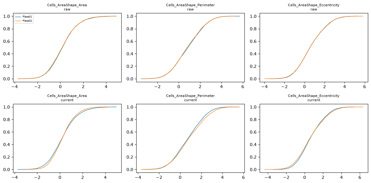
The controls now sit at zero on every plate by construction. keep_raw=True kept the original values in layers["raw"] for the before-and-after plot. It is off by default because the extra layer doubles memory and the original is already on disk.

import matplotlib.pyplot as plt

mt.pl.feature_distributions(adata, features=list(adata.var_names[:3]))
plt.show()

Aggregating to wells

Each well’s profile is the median across its cells. The median is used instead of the mean so that a few extreme cells do not move the profile.

wells = mt.tl.aggregate(adata, by=("Metadata_Plate", "Metadata_Well"), func="median")
wells

AnnData object with n_obs × n_vars = 192 × 80
    obs: 'Metadata_Plate', 'Metadata_Well', 'Metadata_CellCount', 'Metadata_Row', 'Metadata_Col', 'Metadata_Perturbation', 'Metadata_Control', 'Metadata_Batch'
    var: 'object', 'feature_group', 'feature', 'channel', 'scale', 'angle', 'gray_levels', 'radial_bin', 'params', 'is_feature', 'qc_n_nan', 'qc_variance', 'qc_n_unique', 'degenerate_scale'
    uns: 'mantispy'
    layers: None (.X)

The result records its provenance and keeps every metadata column that is constant within a well. Columns that vary within a well, such as a per-cell measurement, are dropped because they have no single value per well.

wells.uns["mantispy"]["aggregated_from"]

{'by': ['Metadata_Plate', 'Metadata_Well'],
 'func': 'median',
 'n_obs': 11339,
 'min_cells': 10}

Metadata_CellCount is added as well. Cell count is a common confounder, and mt.pp.regress_out can remove its influence later.

Looking at the plate

Plate layout artifacts are easiest to see on a plate map.

mt.pl.plate(wells, color=wells.var_names[0])
plt.show()

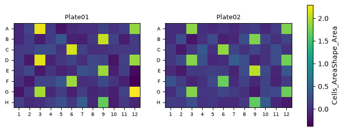
pl.plate draws any feature or obs column, so it also maps per-well flags, for example mt.pl.plate(wells, color="qc_well_pass").

Handing off

get.to_dataframe returns the flat, metadata-first table that pycytominer [Serrano et al., 2025], cytominer-eval and most published scripts expect.

frame = mt.get.to_dataframe(wells)
frame.iloc[:3, :6]

	Metadata_Plate	Metadata_Well	Metadata_CellCount	Metadata_Row	Metadata_Col	Metadata_Perturbation
0	Plate01	A01	60	0	0	DMSO
1	Plate01	A02	60	0	1	pert00
2	Plate01	A03	60	0	2	pert01

Next: 3. Trustworthy profiles, on reducing the features to the informative ones.