11. Concentration response

5. Hits and effects asked whether a treatment moved. This page asks how much of it was needed, which is a different design and a different set of traps:

• Most compounds never plateau inside the tested range, so a four-parameter logistic has no EC50 to find.

• Distance from the controls rises when a compound kills cells, which is not the same finding as a phenotype.

• A dose series usually spends its wells on concentrations rather than replicates, so any single concentration is thinly measured and the evidence lives in the shape across them.

The dataset is the OASIS pilot: 36 compounds over ten concentrations, in two cell lines.

import matplotlib.pyplot as plt
import numpy as np
import pandas as pd
import scanpy as sc

import mantispy as mt

adata = mt.ds.oasis_pilot()
# EMPTY wells hold no compound and no vehicle, so they are neither treatment nor control.
adata = adata[adata.obs["Metadata_Compound"].astype(str) != "EMPTY"].copy()
heparg = adata[adata.obs["Metadata_CellLine"] == "HepaRG"].copy()
heparg

AnnData object with n_obs × n_vars = 2831 × 99
    obs: 'Metadata_plate_map_name', 'Metadata_Plate', 'Metadata_Well', 'Metadata_Site_Count', 'Metadata_Count_Cells', 'Metadata_Count_CellsIncludingEdges', 'Metadata_Count_Cytoplasm', 'Metadata_Count_Nuclei', 'Metadata_Count_NucleiIncludingEdges', 'Metadata_Object_Count', 'Metadata_CellCount', 'Metadata_SiteCount', 'Metadata_Compound', 'Metadata_Concentration', 'Metadata_ConcentrationNominal', 'Metadata_CellLine', 'Metadata_Control', 'Metadata_Perturbation'
    var: 'object', 'feature_group', 'feature', 'channel', 'scale', 'angle', 'gray_levels', 'radial_bin', 'params', 'is_feature'
    uns: 'mantispy'
    layers: None (.X)

The usual preparation

Nothing here is specific to dose response: normalize each plate against its own controls, drop the features with no spread among those controls, then select features.

mt.pp.normalize(heparg, by="Metadata_Plate", reference="negcon")
heparg = heparg[:, ~heparg.var["degenerate_scale"].to_numpy(dtype=bool)].copy()
mt.pp.feature_select(heparg, na_cutoff=0.0)
heparg = mt.pp.subset_features(heparg)
print(f"{heparg.n_obs} wells, {heparg.n_vars} features kept")

2831 wells, 99 features kept

A mantispy object is an AnnData object

Nothing stops scanpy from working on it, which is the point of the format. The PCA, the neighbour graph and the UMAP come from scanpy; the colours come from the columns mt.ds.oasis_pilot attached.

sc.pp.pca(heparg, n_comps=20)
sc.pp.neighbors(heparg)
sc.tl.umap(heparg)

heparg.obs["log10 concentration"] = np.log10(heparg.obs["Metadata_Concentration"].replace(0, np.nan))
sc.pl.umap(heparg, color=["Metadata_Control", "log10 concentration"], size=40, ncols=2, show=False)
plt.tight_layout()

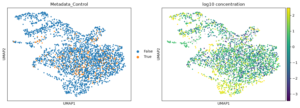
The controls sit together and the highest concentrations sit furthest from them, which is what a dose series should look like before any statistics are run.

From profiles to a response per well

hit_calling() writes two columns. hits_distance is the group’s statistic repeated over its rows; hits_row_distance is each well’s own distance from the control centroid. The curve fit needs the second, because a column that is constant within a group carries no dose information at all.

mt.tl.hit_calling(heparg, groupby="Metadata_Perturbation", use_rep="X_pca", n_permutations=300)
ax = mt.pl.hits(heparg, label_top=6)
plt.show()

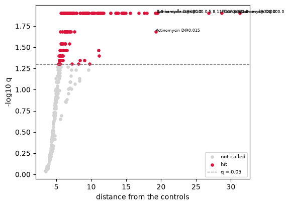
HepaRG carries eight wells at each concentration, so a per-group statistic here rests on eight wells rather than one. That holds only because Metadata_Perturbation is named by Metadata_ConcentrationNominal: two of this accession’s plate maps write the dose to three decimals and the rest to four, and on the raw column a treatment’s wells split across the two spellings. U2OS is two plates rather than eight, and there most groups really do hold one or two wells, which is the trade a plate map makes: concentrations instead of replicates. It is also why the next step is a curve rather than a table of per-concentration tests — a fit reads all ten concentrations together, and the shape across them is what carries the evidence.

Fitting the concentration response

mt.tl.dose_response(heparg, compound_key="Metadata_Compound", dose_key="Metadata_ConcentrationNominal", min_doses=4)
curves = heparg.uns["mantispy"]["dose_response"].set_index("compound")
curves = curves[curves.index.astype(str) != "DMSO"]
curves.sort_values("hitcall", ascending=False).head(8)[
    ["n_doses", "spearman", "qvalue", "ec50", "r_squared", "fit_ok", "hitcall", "hitcall_model"]
]

	n_doses	spearman	qvalue	ec50	r_squared	fit_ok	hitcall	hitcall_model
compound
Staurosporine	11	0.594844	5.546147e-08	2.393946e-01	0.131876	False	1.000000	linear
Fluazinam	11	0.572612	2.002323e-07	1.972621e+01	0.378007	False	1.000000	logistic
Actinomycin D	11	0.430955	1.153459e-04	1.002328e+02	0.106392	False	0.999999	logistic
5,8,11-Eicosatriynoic acid	11	0.387009	6.077550e-04	1.986580e+07	0.481170	False	0.999999	linear
FCCP	11	0.671572	2.577580e-10	2.211261e+08	0.622102	False	0.999999	linear
Cucurbitacin I	11	0.513971	3.047842e-06	3.519991e+01	0.171159	False	0.999998	linear
CLIOQUINOL	11	0.603440	4.385998e-08	7.560393e+01	0.544926	False	0.999998	logistic
5,6-benzoflavone	11	0.513853	3.047842e-06	3.821774e+01	0.614839	False	0.999997	logistic

Three columns answer three different questions, and they disagree on purpose.

spearman with its qvalue asks whether the response rises with dose at all. It assumes no shape and works with three points.

fit_ok asks whether the logistic converged on something curve-shaped with an EC50 inside the tested range. On this screen it is False for most compounds, and that is honest: a compound still climbing at the top concentration has no EC50 in range, so no potency should be quoted for it.

hitcall asks the screener’s question, whether the response is large next to the noise the controls carry. It is the product of three confidences from the ToxCast pipeline: that the curve beats a flat fit, that some concentration’s median clears the cutoff, and that the fitted top clears it. The cutoff is three times the controls’ MAD unless you pass one. hitcall_model names the shape that won: logistic where the curve plateaus, linear where it is still climbing.

fig, axes = plt.subplots(1, 3, figsize=(12, 3.4))
for ax, compound in zip(axes, ["Staurosporine", "Berberine chloride", "MUPIROCIN"], strict=False):
    mt.pl.dose_response(heparg, compound=compound, dose_key="Metadata_ConcentrationNominal", ax=ax)
    ax.set_title(f"{compound} — hit call {curves['hitcall'].get(compound, float('nan')):.2f}")
fig.tight_layout()

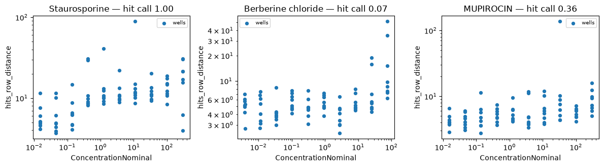
Staurosporine inhibits kinases broadly and climbs far past the band. Mupirocin inhibits a bacterial enzyme and has no target in a human cell, so it never leaves it. Berberine barely leaves it either in this cell line, and the last section says why that is worth checking rather than resolving here.

Distance is not the same as phenotype

A compound that kills cells also moves away from the controls, and the curve cannot tell the two apart. cytotoxicity() compares each group’s cells per field against the controls’, so the calls can be read beside it.

mt.tl.cytotoxicity(heparg, groupby="Metadata_Perturbation")
ax = mt.pl.cytotoxicity(heparg)
plt.show()

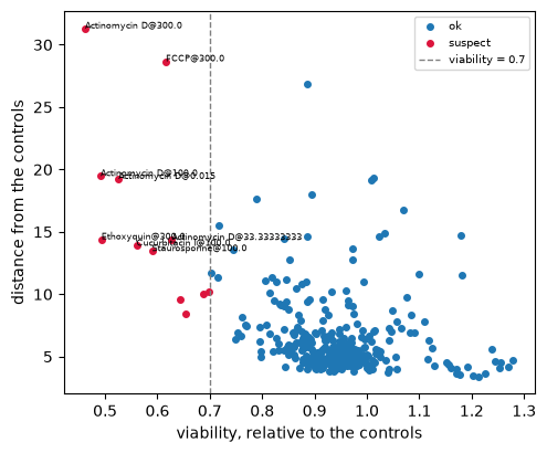
A high call with viability near one is a change in the shape of living cells. A high call with viability collapsed is the morphology of dying cells, which most mechanisms share. The US EPA’s phenotypic profiling pipeline drops any concentration that loses more than half the cells before it fits anything, and that is a reasonable habit here.

Does the call survive a second cell line?

The same compounds were dosed in U2OS. The two lines were normalized and feature-selected apart, so their distances are not on one scale, but their calls can still be compared.

u2os = adata[adata.obs["Metadata_CellLine"] == "U2OS"].copy()
mt.pp.normalize(u2os, by="Metadata_Plate", reference="negcon")
u2os = u2os[:, ~u2os.var["degenerate_scale"].to_numpy(dtype=bool)].copy()
mt.pp.feature_select(u2os, na_cutoff=0.0)
u2os = mt.pp.subset_features(u2os)
sc.pp.pca(u2os, n_comps=20)
mt.tl.hit_calling(u2os, groupby="Metadata_Perturbation", use_rep="X_pca", n_permutations=300)
mt.tl.dose_response(u2os, compound_key="Metadata_Compound", dose_key="Metadata_ConcentrationNominal", min_doses=4)

other = u2os.uns["mantispy"]["dose_response"].set_index("compound")
both = pd.DataFrame({"U2OS": other["hitcall"], "HepaRG": curves["hitcall"]}).dropna()

fig, ax = plt.subplots(figsize=(5, 4.6))
ax.scatter(both["U2OS"], both["HepaRG"], s=30, color="#3a7ca5", zorder=3)
for compound in ["Staurosporine", "Actinomycin D", "Cycloheximide", "MUPIROCIN", "Rifampicin", "Berberine chloride"]:
    if compound in both.index:
        ax.annotate(
            compound,
            (both.loc[compound, "U2OS"], both.loc[compound, "HepaRG"]),
            fontsize=8,
            xytext=(4, 4),
            textcoords="offset points",
        )
ax.axvline(0.9, color="0.8", lw=0.8, zorder=0)
ax.axhline(0.9, color="0.8", lw=0.8, zorder=0)
ax.set(xlabel="hit call in U2OS", ylabel="hit call in HepaRG", xlim=(-0.05, 1.15), ylim=(-0.05, 1.15))
print(
    f"{len(both)} shared compounds, "
    f"{((both['U2OS'] >= 0.9) == (both['HepaRG'] >= 0.9)).mean():.0%} called the same way in both"
)
fig.tight_layout()

28 shared compounds, 57% called the same way in both

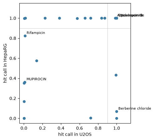
The corners carry the biology. Staurosporine, actinomycin D and cycloheximide inhibit kinases, transcription and translation, and are called in both lines. Mupirocin and rifampicin are antibacterials with no mammalian target, and are called in neither. Berberine sits off the diagonal, called in U2OS and not in HepaRG, which is a statement about two cell types rather than a failure of the fit.

Summary

• Use hits_row_distance as the response, not hits_distance. The group column is one number repeated over its wells.

• fit_ok and hitcall answer different questions. Quote an EC50 only when fit_ok is True; use hitcall to decide whether anything happened at all.

• The cutoff comes from the controls, so a screen with few or drifting controls gives a hit call you should not trust. well_qc() and 8. Trustworthy features and design come first.

• Read every call beside a cell count.

• A call that holds in a second cell line is worth more than a small q-value in one.