6. Mechanism of action

This tutorial runs on BBBC021, the field’s reference benchmark: 38 compounds with published mechanism labels, at one to seven concentrations each, downloaded and cached by mt.ds.bbbc021(). The images are from Caie et al. [2010]; the profiles and the MOA benchmark are from Ljosa et al. [2013].

The questions are whether a profile tells us what a compound does and, where it does not, which mechanisms morphology cannot separate.

import matplotlib.pyplot as plt
import pandas as pd

import mantispy as mt

From wells to one signature per treatment

The recipe is the one from tutorial 4, with one addition. pp.normalize flags features that have no spread among the control wells. mad_robustize divides those by epsilon instead of by zero, so they come back at around 1e17 and dominate every distance computed afterwards. Feature selection does not catch them, because it measures variance across all wells.

BBBC021 has two such features, and dropping them adds 8 points of final accuracy.

adata = mt.ds.bbbc021()
mt.pp.normalize(adata, method="mad_robustize", by="Metadata_Plate", reference="negcon")

degenerate = int(adata.var["degenerate_scale"].sum())
adata = adata[:, ~adata.var["degenerate_scale"].to_numpy()].copy()
mt.pp.feature_select(adata, na_cutoff=0.0)
adata = mt.pp.subset_features(adata)

treated = adata[~adata.obs["Metadata_Control"].to_numpy()].copy()
signatures = mt.tl.consensus(treated, method="median", min_replicates=1)
signatures = signatures[signatures.obs["Metadata_MOA"].notna().to_numpy()].copy()

{
    "features with no spread among the controls": degenerate,
    "features kept": int(adata.n_vars),
    "treatments": int(signatures.n_obs),
    "mechanisms": int(signatures.obs["Metadata_MOA"].nunique()),
}

{'features with no spread among the controls': 2,
 'features kept': 344,
 'treatments': 103,
 'mechanisms': 12}

103 treatments over 12 mechanisms, the shape of the published benchmark.

Classifying

tl.nn_moa_classify assigns each treatment the mechanism of its nearest neighbor. The scheme decides what the number means:

• "nn" allows any neighbor. A compound’s nearest neighbor is usually the same compound at another concentration, so the task reduces to a profile finding its own compound.

• "nsc" (not-same-compound) excludes every neighbor with the same compound. The classifier has to generalize from one molecule to a different one with the same mechanism. The published benchmark uses this rule.

for scheme in ("nn", "nsc"):
    mt.tl.nn_moa_classify(signatures, scheme=scheme, key_added=scheme)

shares = signatures.obs["Metadata_MOA"].value_counts(normalize=True)
{
    "nn accuracy": round(signatures.uns["mantispy"]["nn"]["accuracy"], 3),
    "not-same-compound accuracy": round(signatures.uns["mantispy"]["nsc"]["accuracy"], 3),
    "largest class share (the honest chance level)": round(float(shares.iloc[0]), 3),
}

{'nn accuracy': 0.951,
 'not-same-compound accuracy': 0.777,
 'largest class share (the honest chance level)': 0.136}

The two schemes give 0.95 and 0.78. The nn number mostly measures how well a profile recognizes its own compound at another dose.

Against a largest-class share of 0.14, not-same-compound retrieval of 0.78 is a strong result, and it matches what tutorial 4 computes by hand.

What gets confused with what

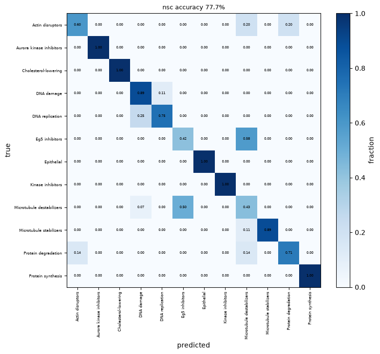
An off-diagonal block in the confusion matrix usually reflects biology.

ax = mt.pl.moa_confusion(signatures, key="nsc")
plt.show()

confusion = signatures.uns["mantispy"]["nsc_confusion"]
confusion[confusion["true"] != confusion["predicted"]].nlargest(5, "count")

	true	predicted	count
5	Eg5 inhibitors	Microtubule destabilizers	7
6	Microtubule destabilizers	Eg5 inhibitors	7
14	DNA replication	DNA damage	2
15	Protein degradation	Actin disruptors	1
16	Protein degradation	Microtubule destabilizers	1

The largest confusion is symmetric and biologically expected: Eg5 inhibitors and microtubule destabilizers, seven treatments each way. Eg5 is the kinesin that separates the centrosomes. Inhibiting it gives a monopolar spindle, and destabilizing microtubules also arrests mitosis. At these doses the two look alike under the microscope, which is a limit of the assay rather than of the classifier.

The second is DNA damage against DNA replication, for the same reason: both stall the cell cycle and both are read out through the DNA channel.

Predicting a hidden mechanism

A blind test is more convincing. For each compound in turn, remove its mechanism label, use tl.moa_enrichment to find what its neighborhood is enriched for, and compare the answer with the removed label. moa_enrichment needs no label on the profile it scores, which is the situation of an uncharacterized compound.

This cell hides each of the 38 compounds in turn, so it is the slowest cell on this page.

compounds = signatures.obs["Metadata_Compound"].astype(str)
truth = signatures.obs.groupby(compounds, observed=True)["Metadata_MOA"].first().astype(str)

records = []
for compound in truth.index:
    blind = signatures.copy()
    blind.obs["Metadata_MOA"] = blind.obs["Metadata_MOA"].astype(str)
    hidden = (blind.obs["Metadata_Compound"].astype(str) == compound).to_numpy()
    blind.obs.loc[hidden, "Metadata_MOA"] = "unknown"

    mt.tl.moa_enrichment(blind, k=10)
    table = blind.uns["mantispy"]["moa_enrichment"]
    asked = set(blind.obs.loc[hidden, "Metadata_Perturbation"].astype(str))
    rows = table[table["group"].isin(asked) & (table["moa"] != "unknown")]
    if rows.empty:
        continue
    predicted = rows.groupby("moa")["pvalue"].min().idxmin()
    records.append({"compound": compound, "true": truth[compound], "predicted": predicted})

blind_test = pd.DataFrame(records)
blind_test["correct"] = blind_test["true"] == blind_test["predicted"]
{
    "compounds tested": len(blind_test),
    "mechanism recovered": int(blind_test["correct"].sum()),
    "rate": round(float(blind_test["correct"].mean()), 3),
}

{'compounds tested': 38, 'mechanism recovered': 26, 'rate': 0.684}

blind_test[~blind_test["correct"]]

	compound	true	predicted	correct
0	ALLN	Protein degradation	Protein synthesis	False
2	AZ-C	Eg5 inhibitors	Microtubule destabilizers	False
4	AZ-U	Epithelial	Protein synthesis	False
8	MG-132	Protein degradation	Microtubule stabilizers	False
11	alsterpaullone	Kinase inhibitors	DNA damage	False
14	camptothecin	DNA replication	DNA damage	False
17	colchicine	Microtubule destabilizers	DNA damage	False
19	cytochalasin B	Actin disruptors	Protein synthesis	False
20	cytochalasin D	Actin disruptors	Protein synthesis	False
25	etoposide	DNA damage	DNA replication	False
27	lactacystin	Protein degradation	Eg5 inhibitors	False
28	latrunculin B	Actin disruptors	Protein synthesis	False

Two thirds of the compounds have their mechanism recovered from morphology alone, without the label, against a chance level of 0.14.

The failures fall into three groups.

Some repeat the confusion matrix. Etoposide and camptothecin swap DNA damage and DNA replication in both directions, and AZ-C, an Eg5 inhibitor, is predicted as a microtubule destabilizer. A mechanism that is hard for the nearest-neighbor rule is also hard for the neighborhood test, so the two methods are consistent.

Some are a whole class. All three actin disruptors miss, each predicted as protein synthesis, so at these concentrations the actin phenotype does not separate that class in this assay. All three protein-degradation compounds miss as well: ALLN, MG-132 and lactacystin, three proteasome inhibitors with three different wrong answers. That is the largest failure on the page, and it does not appear among the confusion matrix’s top pairs because the errors are spread out. A class that fails in three different directions has no consistent readout in this assay, which says more than a single confused pair.

One is unexpected: colchicine, a standard microtubule destabilizer, is predicted as DNA damage. Look at its images before drawing further conclusions about it.

Which measurements separate the mechanisms

var already records which object, measurement family and channel each feature belongs to. tl.feature_sets turns that into a decoupler network, and tl.enrich scores every signature against every set, so the result says which kinds of measurement moved instead of which individual features.

BBBC021’s three channels are DAPI, tubulin and actin. The feature names spell them CorrDAPI, CorrTub and CorrActin (the Corr prefix marks CellProfiler’s illumination-corrected image, and the parser keeps the names as they are), and the table below uses those names. If the enrichment carries signal, the tubulin-directed mechanisms should load on the tubulin channel.

mt.tl.enrich(signatures, by="group_by_channel", method="ulm", tmin=5)
mt.tl.rank_sets(signatures, groupby="Metadata_MOA")

ranked = signatures.uns["mantispy"]["rank_sets"]
top = (
    ranked.sort_values("score", ascending=False)
    .groupby("group", observed=True)
    .head(2)
    .sort_values(["group", "score"], ascending=[True, False])
)
top.round(2)

	group	set	score
56	Actin disruptors	Intensity|CorrTub	3.12
55	Actin disruptors	Intensity|CorrDAPI	1.67
7	Aurora kinase inhibitors	Intensity|CorrDAPI	0.96
10	Aurora kinase inhibitors	Texture|CorrDAPI	0.11
69	Cholesterol-lowering	Texture|CorrActin	3.04
70	Cholesterol-lowering	Texture|CorrDAPI	2.99
46	DNA damage	Texture|CorrDAPI	0.10
47	DNA damage	Texture|CorrTub	-0.51
41	DNA replication	Texture|CorrTub	0.78
40	DNA replication	Texture|CorrDAPI	-1.14
12	Eg5 inhibitors	Intensity|CorrActin	3.84
14	Eg5 inhibitors	Intensity|CorrTub	1.65
22	Epithelial	Texture|CorrDAPI	1.29
23	Epithelial	Texture|CorrTub	0.83
29	Kinase inhibitors	Texture|CorrTub	1.18
28	Kinase inhibitors	Texture|CorrDAPI	1.11
48	Microtubule destabilizers	Intensity|CorrActin	3.13
51	Microtubule destabilizers	Texture|CorrActin	0.76
62	Microtubule stabilizers	Intensity|CorrTub	3.10
60	Microtubule stabilizers	Intensity|CorrActin	0.40
2	Protein degradation	Intensity|CorrTub	2.84
0	Protein degradation	Intensity|CorrActin	0.59
32	Protein synthesis	Intensity|CorrTub	4.47
31	Protein synthesis	Intensity|CorrDAPI	1.78

ax = mt.pl.sets_heatmap(signatures, groupby="Metadata_MOA", top=20)
plt.show()

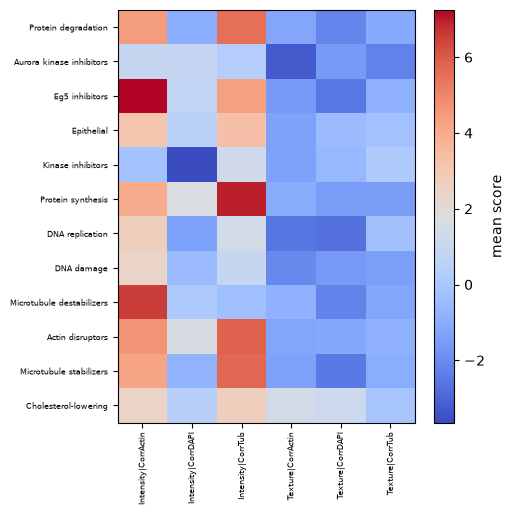
Microtubule stabilizers load most strongly on tubulin intensity. The pipeline was never told which channel stains microtubules; the channel comes from parsing the feature names, as in tutorial 1. This result therefore also checks the annotation.

The mapping is not one-to-one. Actin disruptors also score highest on tubulin intensity, and Eg5 inhibitors on actin. The two cytoskeletal systems are mechanically coupled, and a cell whose actin has collapsed looks different in every channel. Read the enrichment as which measurements changed, not as which protein was targeted.

Distances between mechanisms

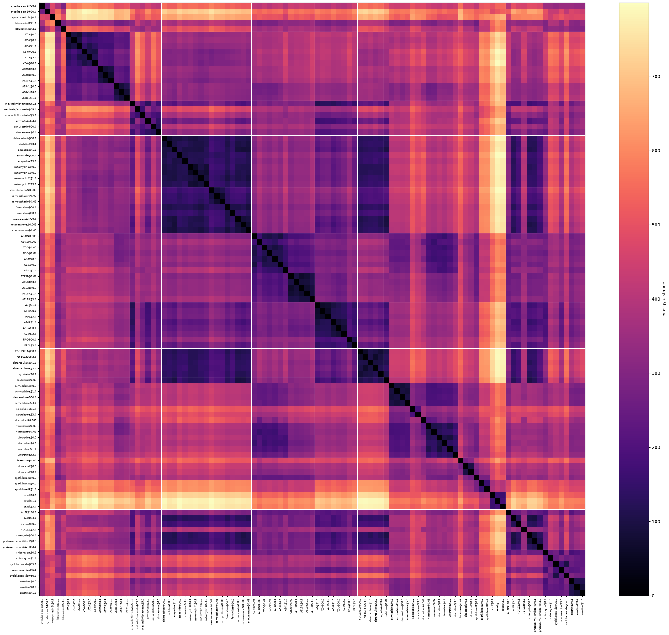
tl.edistance with reference=None gives the full treatment-by-treatment energy distance matrix, and pl.distance_heatmap orders it by mechanism so related treatments sit together.

mt.tl.edistance(signatures, reference=None)
ax = mt.pl.distance_heatmap(signatures, groupby="Metadata_MOA")
plt.show()

Summary

• Report the not-same-compound number, or state which rule you used. The gap between the two is large enough to change conclusions.

• Chance is the largest class’s share, not one over the number of classes.

• Confusions are hypotheses about the assay. The confusion between Eg5 inhibitors and microtubule destabilizers shows what these images can resolve.

• moa_enrichment scores a compound without a label, as needed in a screen of uncharacterized molecules.

Next: single-cell heterogeneity, on what a well median hides.