3. Trustworthy profiles

A CellProfiler run gives you a few thousand features, and most are redundant. AreaShape_Area and AreaShape_Perimeter carry much the same information, and so does a texture feature at scale 3 and the same texture at scale 5. Others are constant, or blow up because they are ratios with a near-zero denominator.

Feature selection removes these. mantispy reproduces pycytominer’s operations [Serrano et al., 2025], verified feature by feature, because published pipelines depend on their precise behavior.

import matplotlib.pyplot as plt

import mantispy as mt

cells = mt.ds.synthetic_plate(
    n_plates=2,
    n_wells=96,
    n_cells=30,
    n_features=60,
    n_correlated_pairs=8,
    n_constant_features=4,
    effect_size=2.0,
    seed=0,
)
mt.pp.normalize(cells, by="Metadata_Plate", reference="negcon")
wells = mt.tl.aggregate(cells)
{"wells x features": wells.shape, "flagged degenerate_scale": int(wells.var["degenerate_scale"].sum())}

{'wells x features': (192, 68), 'flagged degenerate_scale': 4}

normalize warned and flagged four features in var["degenerate_scale"]. These are the constant features the generator injected. They have no spread among the control wells, so mad_robustize divides them by epsilon = 1e-18 instead of by zero, as pycytominer does, and they come back at around 1e17.

Here the variance threshold below removes them. It cannot catch a feature that varies across the plate but is constant among the few control wells: feature selection measures variance across all wells, keeps that feature, and it then dominates every distance computed afterwards. Whenever var["degenerate_scale"] flags anything, drop those columns before selecting:

adata = adata[:, ~adata.var["degenerate_scale"].to_numpy()].copy()

On BBBC021 that is two features out of 473, and dropping them adds eight points of mechanism retrieval (see tutorial 6).

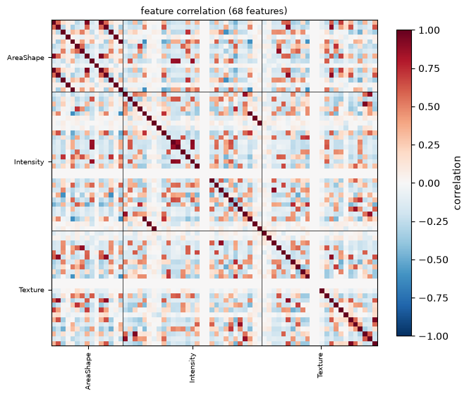
The generator injected eight near-duplicate feature pairs and four constant features, so we can check that selection removes them. n_correlated_pairs=8 adds a partner for eight of the features, so the object has 68 columns instead of the 60 requested, and every count below is out of 68.

Before

The correlation heatmap is ordered by feature group, with a line at each group boundary. Blocks along the diagonal are families of features that measure nearly the same thing.

mt.pl.feature_correlation(wells, key=None)
plt.show()

The operations

Each operation tests one criterion, and feature_select combines them. It does not drop anything: it writes a boolean column to var, and only subset_features changes the shape, so you can inspect what would be removed first.

operation	drops a feature when
variance_threshold	its variance is below min_variance
frequency_threshold	one value dominates it, or it takes very few distinct values
correlation_threshold	it is highly correlated with another feature
drop_na_columns	too much of it is missing
blocklist	it is on the CellProfiler blocklist of known-unreliable features
drop_outliers	its magnitude has blown up
noise_removal	it varies too much between replicates of the same perturbation

Two of these are easy to get wrong.

variance_threshold is a plain variance cut. The frequency-and-uniqueness rule often described under that name is a separate operation, frequency_threshold, and its two criteria combine with OR.

correlation_threshold uses the signed correlation, not the absolute value, so two features correlated at −1.0 are both kept. pycytominer does the same, and mantispy matches it.

for operation in ("variance_threshold", "correlation_threshold", "blocklist", "drop_na_columns"):
    trial = wells.copy()
    mt.pp.feature_select(trial, operations=(operation,))
    print(f"{operation:24s} keeps {int(trial.var['selected'].sum()):3d} of {trial.n_vars}")

variance_threshold       keeps  64 of 68
correlation_threshold    keeps  56 of 68
blocklist                keeps  68 of 68
drop_na_columns          keeps  68 of 68

blocklist and drop_na_columns keep everything here. The blocklist names real CellProfiler features, and these synthetic ones are not on it. This generator call also injected no missing values. On a real plate both remove features.

Running the default pipeline

The default runs four of the seven operations. frequency_threshold and drop_outliers are off because both can remove an informative feature on a screen with few conditions. noise_removal is off because it needs replicate structure, which not every object has.

mt.pp.feature_select(wells)
wells.uns["mantispy"]["feature_select"]

{'variance_threshold': 4,
 'correlation_threshold': 12,
 'drop_na_columns': 0,
 'blocklist': 0}

survivors = set(wells.var_names[wells.var["selected"]])
constant = wells.uns["mantispy"]["truth"]["constant_features"]
pairs = wells.uns["mantispy"]["truth"]["correlated_pairs"]

{
    "constant features kept": [name for name in constant if name in survivors],
    "duplicate pairs left intact": [(a, b) for a, b in pairs if {a, b} <= survivors],
}

{'constant features kept': [], 'duplicate pairs left intact': []}

Every constant feature is gone, and no near-duplicate pair survived intact.

selected = mt.pp.subset_features(wells)
mt.pl.feature_correlation(selected, key=None)
plt.show()

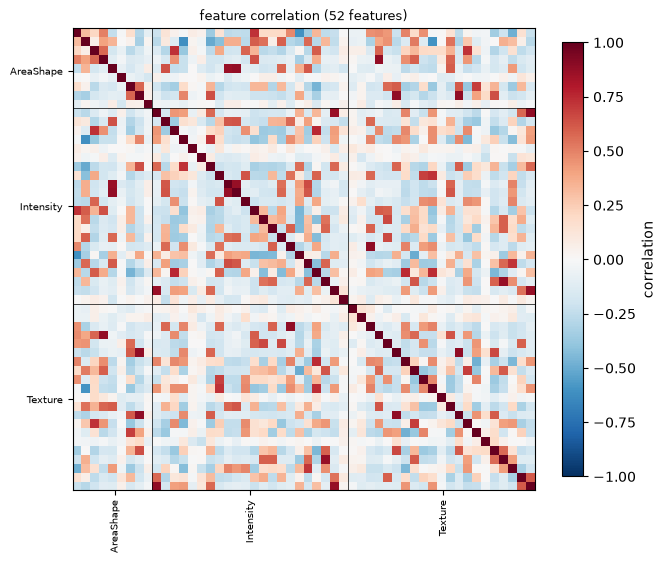
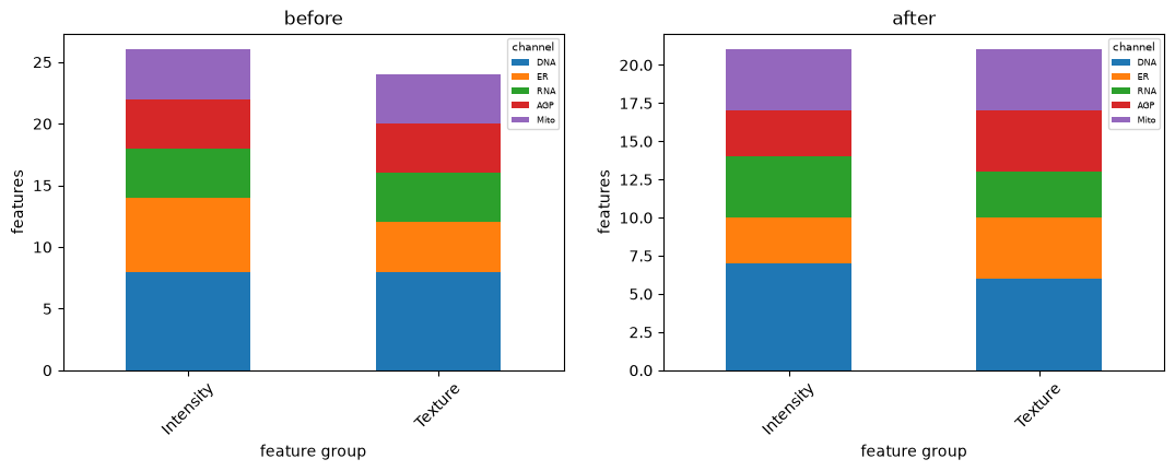
The blocks are gone. pl.feature_groups shows which feature families lost features to selection.

fig, axes = plt.subplots(1, 2, figsize=(13, 4))
mt.pl.feature_groups(wells, ax=axes[0])
axes[0].set_title("before")
mt.pl.feature_groups(wells, key="selected", ax=axes[1])
axes[1].set_title("after")
plt.show()

The blocklist

The default blocklist is pycytominer’s, copied unchanged with its source recorded in the file. It lists features known to be unreliable: twenty Manders and twenty rank-weighted colocalization coefficients, plus the three highest granularity bands. MeasureColocalization writes Manders, RWC and Costes coefficients, and only the first two are on the list.

from mantispy._core.features import load_blocklist

blocked = load_blocklist()
len(blocked), blocked[:3]

(55,
 ['Nuclei_Correlation_Manders_AGP_DNA',
  'Nuclei_Correlation_Manders_AGP_ER',
  'Nuclei_Correlation_Manders_AGP_Mito'])

Outlying cells

Feature selection cleans the columns, and outlier detection cleans the rows. A segmentation failure, a clump of debris or a dying cell gives an extreme profile that says nothing about the perturbation.

This section uses real cells. jump_cells() holds about 13,600 cells from 24 wells of one JUMP plate [Chandrasekaran et al., 2023], as CellProfiler measured them. The first call downloads about 1.5 GB.

import numpy as np
import pandas as pd

jump = mt.ds.jump_cells()
mt.pp.outliers(jump, contamination=0.02)
mt.pl.outliers(jump, groupby="Metadata_Well")
plt.show()

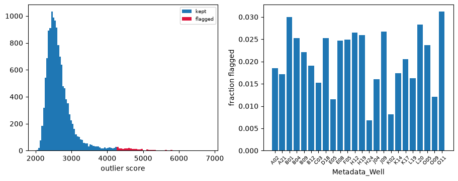
outliers() writes a flag and a score and removes nothing. The histogram shows the flagged tail of the score, and the bars the fraction flagged in each well. It scores only the features var["selected"] marks, so a block of near-duplicate features cannot outvote the rest.

The default method, ecod [Li et al., 2023], needs no tuning. A cell’s score is the sum over features of how far into a tail it sits, measured by rank, so the scale of a feature does not matter. isolation_forest catches cells that are unusual in their combination of features, and mad takes the largest robust z-score of any single feature, so score_cutoff=5 applies the usual five-robust-standard-deviations rule instead of a fixed fraction.

What gets flagged

Three measurements that are easy to picture, as percentiles within the plate:

features = ["Cells_AreaShape_Area", "Nuclei_AreaShape_Area", "Nuclei_Intensity_MeanIntensity_DNA"]
percentiles = mt.get.to_dataframe(jump, metadata=False, features=features).rank(pct=True)
percentiles.groupby(jump.obs["qc_outlier"]).median().round(2)

	Cells_AreaShape_Area	Nuclei_AreaShape_Area	Nuclei_Intensity_MeanIntensity_DNA
qc_outlier
False	0.51	0.51	0.49
True	0.06	0.07	0.97

Flagged cells are small, with small nuclei and bright DNA. Rounded cells look like that: cells in division, dying cells and fragments. Two fields of well O09 were imaged as well, and jump_plate() downloads them (44 MB), so the flagged cells there can be set beside cells that were kept. DNA is red, AGP green and Mito blue, and the white line is CellProfiler’s outline of the cell.

from spatialdata import get_pyramid_levels

plate = mt.ds.jump_plate()
imaged = jump.obs[(jump.obs["Metadata_Well"] == "O09") & jump.obs["Metadata_Site"].isin([1, 2])]
examples = {
    "flagged": imaged[imaged["qc_outlier"]].head(4),
    "kept": imaged[~imaged["qc_outlier"]].sample(4, random_state=0),
}

fig, axes = plt.subplots(2, 4, figsize=(10, 5))
for row, (label, cells_shown) in zip(axes, examples.items(), strict=True):
    row[0].set_title(label, loc="left")
    for ax, (_, cell) in zip(row, cells_shown.iterrows(), strict=False):
        field = f"BR00121438_O09_s{cell['Metadata_Site']}"
        mask = np.asarray(plate[f"{field}_cells"]) == cell["Metadata_ObjectNumber"]
        ys, xs = np.nonzero(mask)
        window = np.s_[max(ys.min() - 15, 0) : ys.max() + 15, max(xs.min() - 15, 0) : xs.max() + 15]
        image = get_pyramid_levels(plate[f"{field}_image"], n=0)
        rgb = np.stack([np.asarray(image.sel(c=c))[window] for c in ("DNA", "AGP", "Mito")], axis=-1).astype(float)
        ax.imshow((rgb / np.percentile(rgb, 99.5, axis=(0, 1))).clip(0, 1))
        ax.contour(mask[window], levels=[0.5], colors="white", linewidths=0.8)
for ax in axes.flat:
    ax.set_axis_off()
plt.show()

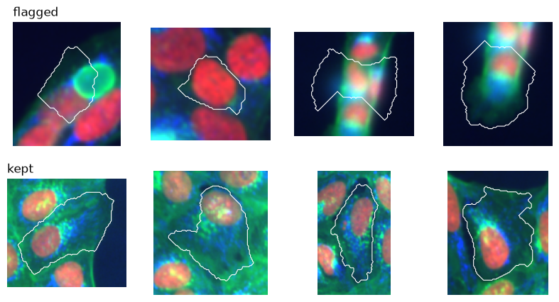
The kept cells are flat and spread out. The flagged ones are rounded, out of focus and badly outlined: the first outline covers the space beside a round cell rather than the cell, the second holds little but a nucleus, and the last two cut across a column of rounded cells. Their profiles describe the segmentation more than the cell.

The methods disagree

flags = {"ecod": jump.obs["qc_outlier"].to_numpy()}
for name, kwargs in {
    "ecod, paper": {"ecod_aggregation": "paper"},
    "isolation_forest": {"method": "isolation_forest"},
    "mad": {"method": "mad"},
}.items():
    mt.pp.outliers(jump, contamination=0.02, key_added="qc_compare", **kwargs)
    flags[name] = jump.obs["qc_compare"].to_numpy()

pd.DataFrame({a: {b: (flags[a] & flags[b]).sum() / (flags[a] | flags[b]).sum() for b in flags} for a in flags}).round(2)

	ecod	ecod, paper	isolation_forest	mad
ecod	1.00	0.79	0.83	0.21
ecod, paper	0.79	1.00	0.79	0.21
isolation_forest	0.83	0.79	1.00	0.22
mad	0.21	0.21	0.22	1.00

The table is the Jaccard index between flagged sets. ecod and isolation_forest flag largely the same cells. mad flags mostly others, because one extreme feature is enough for it. ecod_aggregation="paper" scores as Algorithm 1 of Li et al. [2023] does rather than as pyod does, and on these cells it shares most of its flags with the default.

Is it removing a phenotype?

per_well = jump.obs.groupby("Metadata_Well", observed=True).agg(
    control=("Metadata_Control", "first"), flagged=("qc_outlier", "mean")
)
per_well.groupby("control")["flagged"].agg(["count", "min", "median", "max"]).round(3)

	count	min	median	max
control
False	16	0.007	0.021	0.030
True	8	0.011	0.022	0.031

Control and compound wells lose the same fraction, from under 1 % to 3 % of a well, so here the flags fall on every well alike rather than on one compound’s response. On a plate with a strong phenotype they may not: a compound that stops cells in division fills its wells with exactly the rounded cells flagged above. Look at this table before dropping anything. If one perturbation’s wells stand out, pass by="Metadata_Well" so each well is compared only with itself, or keep the cells.

Diagnostics

Run these two plots before any correction. They show whether you need one.

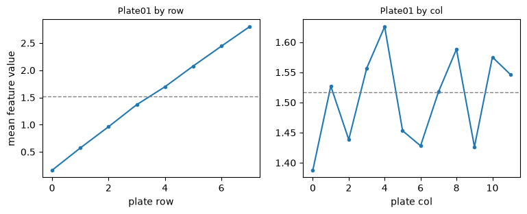
plate_effects shows row and column marginals per plate. A position artifact appears as a trend across rows or columns, while noise scatters around the plate median.

gradient = mt.ds.synthetic_plate(n_wells=96, n_cells=10, n_features=20, row_gradient=3.0, seed=0)
mt.pl.plate_effects(mt.tl.aggregate(gradient, min_cells=0))
plt.show()

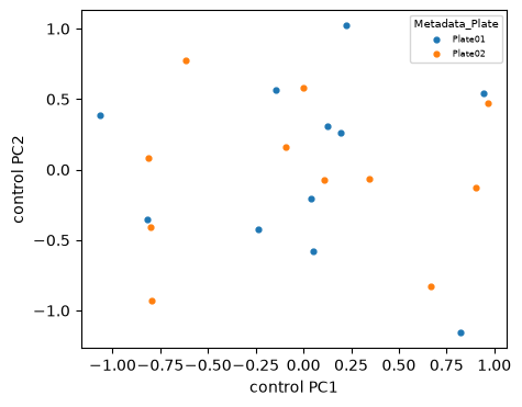
control_drift projects the control wells onto components fitted on the controls alone. If the controls of different plates land in different places, the reference itself shifts between plates, which is what normalization should remove.

mt.pl.control_drift(wells, groupby="Metadata_Plate")
plt.show()

Next: 4. Correcting and evaluating, on removing these artifacts and measuring whether that helped.