8. Trustworthy features and experimental design

This page covers four questions that come up in most screens:

• which features can I trust?

• how much of what I see is batch effect?

• how many replicates do I need?

• is this hit real, or did the compound kill the cells?

BBBC021 is used for the first three. The fourth uses a synthetic plate, where which perturbation lost its cells is known in advance.

import matplotlib.pyplot as plt
import numpy as np

import mantispy as mt

The recipe from tutorial 6, including the degenerate_scale drop it explains.

adata = mt.ds.bbbc021()
mt.pp.normalize(adata, method="mad_robustize", by="Metadata_Plate", reference="negcon")
adata = adata[:, ~adata.var["degenerate_scale"].to_numpy()].copy()
mt.pp.feature_select(adata, na_cutoff=0.0)
adata = mt.pp.subset_features(adata)

treated = adata[~adata.obs["Metadata_Control"].to_numpy()].copy()
treated.shape

(302, 344)

Which features can I trust?

A feature with high variance can still be useless. If that variance lies within replicates of the same treatment rather than between treatments, it is noise. A variance filter cannot tell the difference because it ignores the replicate structure.

pp.feature_reproducibility computes the intraclass correlation (ICC), the share of a feature’s variance that lies between replicate groups.

mt.pp.feature_reproducibility(treated, groupby="Metadata_Perturbation")
icc = treated.var["icc"]
{
    "median": round(float(icc.median()), 3),
    "lower quartile": round(float(icc.quantile(0.25)), 3),
    "upper quartile": round(float(icc.quantile(0.75)), 3),
    "features above 0.2": int((icc > 0.2).sum()),
    "of": int(treated.n_vars),
}

{'median': 0.38,
 'lower quartile': 0.203,
 'upper quartile': 0.537,
 'features above 0.2': 261,
 'of': 344}

Does selecting on ICC help? The answer differs between two retrieval tasks.

Replicate retrieval, whether a treatment’s replicates find each other, is what mAP measures.

def replicate_map(profiles):
    """Mean average precision of replicate retrieval."""
    scratch = profiles.copy()
    mt.tl.map(scratch, mode="replicability", null_size=500, seed=0)
    return float(scratch.uns["mantispy"]["map"]["mean_average_precision"].mean())


{
    "all features": round(replicate_map(treated), 3),
    "ICC > 0.2": round(replicate_map(treated[:, (icc > 0.2).to_numpy()].copy()), 3),
    "ICC > 0.4": round(replicate_map(treated[:, (icc > 0.4).to_numpy()].copy()), 3),
}

{'all features': 0.323, 'ICC > 0.2': 0.349, 'ICC > 0.4': 0.375}

Replicate retrieval improves clearly. The same filter improves it on the other two packaged screens as well (measured separately, not on this page): rohban goes from 0.138 to 0.190 and pki from 0.252 to 0.261. In relative terms rohban gains the most of the three (+38% against +8% for BBBC021) and pki the least, so the size of the gain depends on the screen and has to be measured.

Mechanism retrieval, whether a compound finds a different compound with the same mechanism, is the task from tutorial 6. Here the same filter does not help.

def not_same_compound(profiles):
    """Not-same-compound mechanism retrieval, as in tutorial 6."""
    signatures = mt.tl.consensus(profiles.copy(), method="median", min_replicates=1)
    signatures = signatures[signatures.obs["Metadata_MOA"].notna().to_numpy()].copy()
    mt.tl.nn_moa_classify(signatures, scheme="nsc")
    return float(signatures.uns["mantispy"]["moa"]["accuracy"])


{
    "all features": round(not_same_compound(treated), 3),
    "ICC > 0.2": round(not_same_compound(treated[:, (icc > 0.2).to_numpy()].copy()), 3),
    "ICC > 0.4": round(not_same_compound(treated[:, (icc > 0.4).to_numpy()].copy()), 3),
}

{'all features': 0.777, 'ICC > 0.2': 0.767, 'ICC > 0.4': 0.757}

Reproducible and generalizable are different properties. ICC favors features whose replicates agree, which is what replicate retrieval rewards. Transferring from one molecule to another with the same mechanism needs something else, and filtering on reproducibility slightly hurts it here.

Use ICC when the question is reproducibility. For other tasks, measure its effect first, and choose the cutoff from the ICC distribution instead of using a default.

How much of this is batch effect?

pp.feature_batch_sensitivity tests each feature for dependence on batch with a Kruskal-Wallis test and corrects for multiple testing across features. Run it after any correction you applied, to see what batch dependence remains.

mt.pp.feature_batch_sensitivity(treated, batch_key="Metadata_Plate")
{
    "plates": int(treated.obs["Metadata_Plate"].nunique()),
    "features still plate-dependent at q < 0.05": int(treated.var["batch_sensitive"].sum()),
    "of": int(treated.n_vars),
}

{'plates': 49, 'features still plate-dependent at q < 0.05': 338, 'of': 344}

Nearly every feature depends on batch after per-plate normalization. Centering each plate on its own controls removes the plate’s offset, but not differences in how features respond within the plate.

Treat this as a warning against interpreting small effects across plates. Compare a corrected run with an uncorrected one to see whether the count drops, and evaluate corrections with mt.metrics.evaluate_correction.

How many replicates do I need?

tl.replicate_saturation subsamples replicates and reports how much the signature still changes at each depth. There are two metrics, and the number of replicates in the screen decides which one applies:

• "signature_stability" correlates two disjoint subsets. It is unbiased and needs 2 * depth replicates.

• "convergence" correlates a subset with the group’s full signature. It is defined up to one less than the group size and is optimistic by construction.

BBBC021 has three replicates per treatment, so the unbiased measure gives a single point.

mt.tl.replicate_saturation(treated, metric="convergence", n_draws=10)
treated.uns["mantispy"]["replicate_saturation"].round(3)

	n_replicates	mean	std	n_draws
0	1	0.793	0.009	10
1	2	0.873	0.004	10

ax = mt.pl.replicate_saturation(treated)
plt.show()

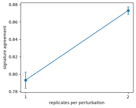
From one replicate to two, signature agreement rises from 0.79 to 0.87 and is still rising at the largest depth the data supports. For an experiment that has to distinguish mechanisms, three replicates is on the low side, which is useful when planning the next screen.

Is it a hit, or did the cells die?

A compound that kills four fifths of the cells leaves a well median computed from a fifth as many cells, and that median moves away from the controls for reasons unrelated to the biology being screened. It looks like a strong hit.

The cell count is also a baseline to beat. Seal et al. [2025] found that across three bioactivity benchmarks a model given only the cell count often matched one given the whole Cell Painting profile, and Ewald et al. [2026] found that profiles predicted LDH release no better than cell count, plate and well position.

So that the answer is known in advance, this section uses a synthetic plate where one perturbation is purely cytotoxic: 80% of its cells are removed and its injected morphology effect is subtracted again. Only the cell loss remains.

plate = mt.ds.synthetic_plate(n_wells=192, n_cells=50, n_features=25, n_perturbations=3, effect_size=3.0, seed=0)
rng = np.random.default_rng(0)

toxic = (plate.obs["Metadata_Perturbation"] == "pert02").to_numpy()
plate = plate[~toxic | (rng.random(plate.n_obs) < 0.2)].copy()

rows = (plate.obs["Metadata_Perturbation"] == "pert02").to_numpy()
values = plate.X.copy()
for name in plate.uns["mantispy"]["truth"]["affected_features"]["pert02"]:
    column = list(plate.var_names).index(name)
    values[rows, column] -= values[rows, column].mean() - values[~rows, column].mean()
plate.X = values

mt.pp.normalize(plate, by="Metadata_Plate", reference="negcon")
wells = mt.tl.aggregate(plate, min_cells=0)
mt.tl.hit_calling(wells, n_permutations=500)
wells.uns["mantispy"]["hits"][["group", "distance", "qvalue", "is_hit"]].round(3)

	group	distance	qvalue	is_hit
0	DMSO	284.522	0.130	False
1	pert00	2831.307	0.003	True
2	pert01	2414.603	0.003	True
3	pert02	661.269	0.003	True

pert02 has no morphology effect left and is still called a hit, at 661 against 285 for the controls. Hit calling cannot tell the difference, because nothing in the profile says why it moved. (The covariance warning is the one explained in tutorial 5: 24 control rows for 25 features. It affects the scale of these distances, not their order.)

mt.tl.cytotoxicity(wells)
wells.uns["mantispy"]["cytotoxicity"].round(3)

	group	n_obs	viability	distance	suspect
0	DMSO	48	1.0	78.961	False
1	pert00	48	1.0	2831.307	False
2	pert01	48	1.0	2414.603	False
3	pert02	48	0.2	661.269	True

ax = mt.pl.cytotoxicity(wells)
plt.show()

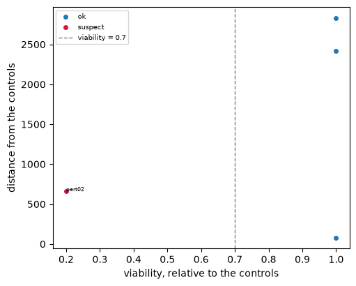
pert02 has a viability of 0.20 and is the only group flagged. The two perturbations with real effects and no cell loss are not flagged.

Both conditions have to hold. Cell loss alone is a phenotype (a compound that arrests growth is a real finding), and a large distance alone is a hit. Only the combination is suspect.

How much this matters depends on the screen. Measured separately on the other two packaged screens, the rank correlation between phenotype distance and cell loss is +0.79 over the pki dose series and +0.00 over rohban’s ORF overexpression. tl.cytotoxicity is a diagnostic and does not correct anything.

Genetic screens: does the screen recover known biology?

When the perturbation is a gene rather than a compound, gene-set resources apply. tl.gene_sets fetches one through decoupler, and tl.pathway_coherence tests whether the genes of a set produce similar morphologies, against a null of random sets of the same size.

This needs a Metadata_Gene column, so it does not apply to BBBC021. rohban has Metadata_GeneID and Metadata_Perturbation. Either can be copied into Metadata_Gene; the snippet below uses the perturbation because consensus groups on it:

genes = mt.tl.consensus(rohban, method="median", min_replicates=2)
genes.obs["Metadata_Gene"] = genes.obs["Metadata_Perturbation"].astype(str).to_numpy()

net = mt.tl.gene_sets("hallmark")
mt.tl.pathway_coherence(genes, net, min_genes=4)
mt.pl.pathway_coherence(genes)

Run this way (measured separately, not on this page), hallmark covers 133 of the screen’s 190 genes, and 29 sets have enough members to score. No set passes FDR; the most coherent is COMPLEMENT at q = 0.51. At this power the screen does not recover hallmark program structure. Hallmark sets are transcriptional programs, and the test asks whether overexpressing genes from the same program produces similar morphology, which need not be the case.

The table is sorted by coherence, not by p-value. With a permutation null every coherent set ties at the smallest possible p-value, so the p-value shows whether a set is coherent and the statistic ranks the sets.

Summary

• Reproducibility and generalizability are different properties, and a filter that improves one can hurt the other. Measure the task you care about.

• Per-plate normalization does not remove all plate structure. Check what remains.

• A saturation curve that is still rising says the next experiment needs more replicates.

• Cell loss and phenotype are confounded by construction. Flag the combination instead of correcting it away.

Next: 9. Scaling up, and correcting across laboratories, on data that does not fit in memory and data from two laboratories.