OASIS pilot

Thirty-six compounds over a ten-point dose range, run in U2OS and in HepaRG, plus two batches of assay development: cpg0033-oasis-pilot on the Cell Painting Gallery [Weisbart et al., 2024].

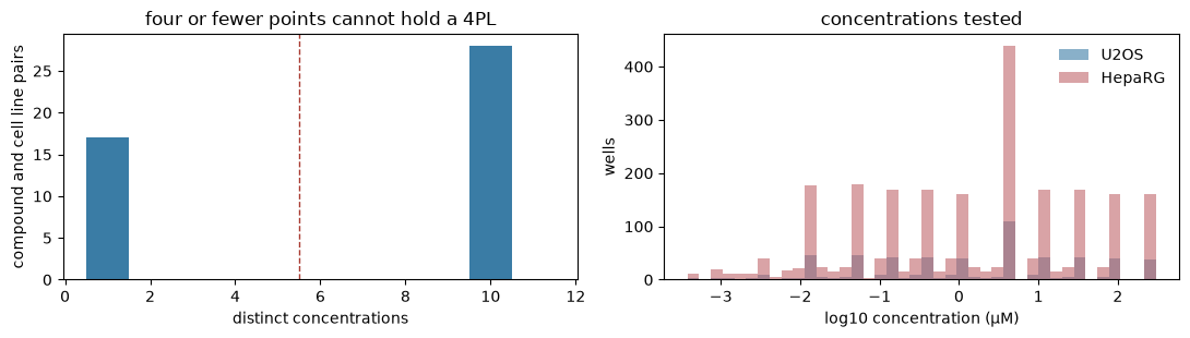
It is the dose-response dataset of the package. Every other pinned dataset either fixes one concentration per compound or, like BBBC021, keeps only the handful of doses its mechanism benchmark needed. A four-parameter curve has five things to estimate, so three or four concentrations leave it underdetermined and dose_response() can report a potency that the data does not support. Here 28 compounds carry six or more concentrations in each of two cell lines, so a curve has something to hold on to and every compound can be read twice in two different biological backgrounds.

import matplotlib.pyplot as plt
import numpy as np
import pandas as pd

import mantispy as mt

adata = mt.ds.oasis_pilot()
adata

AnnData object with n_obs × n_vars = 4604 × 99
    obs: 'Metadata_plate_map_name', 'Metadata_Plate', 'Metadata_Well', 'Metadata_Site_Count', 'Metadata_Count_Cells', 'Metadata_Count_CellsIncludingEdges', 'Metadata_Count_Cytoplasm', 'Metadata_Count_Nuclei', 'Metadata_Count_NucleiIncludingEdges', 'Metadata_Object_Count', 'Metadata_CellCount', 'Metadata_SiteCount', 'Metadata_Compound', 'Metadata_Concentration', 'Metadata_ConcentrationNominal', 'Metadata_CellLine', 'Metadata_Control', 'Metadata_Perturbation'
    var: 'object', 'feature_group', 'feature', 'channel', 'scale', 'angle', 'gray_levels', 'radial_bin', 'params', 'is_feature'
    uns: 'mantispy'
    layers: None (.X)

Source

file	from	holds
<plate>_normalized_feature_select_batch.csv.gz	cpg0033-oasis-pilot/broad/workspace/profiles	the well-level profiles, normalized and feature-selected per batch upstream
<plate>.txt	cpg0033-oasis-pilot/broad/workspace/metadata/<batch>/platemap	the plate map: which compound sits in which well, and at what concentration

Twelve plates over four batches, read down to the 99 features they share. Columns are intersected because the batches were feature-selected separately, which is the first thing to keep in mind: the two cell lines were processed apart, so a distance computed in one is not on the same scale as a distance in the other.

obs = adata.obs
per_plate = obs.groupby(["Metadata_CellLine", "Metadata_Plate"], observed=True).agg(
    wells=("Metadata_Well", "size"),
    DMSO=("Metadata_Control", "sum"),
    empty=("Metadata_Compound", lambda column: int((column.astype(str) == "EMPTY").sum())),
    compounds=("Metadata_Compound", lambda column: column[~column.astype(str).isin(["DMSO", "EMPTY"])].nunique()),
    median_cells=("Metadata_CellCount", "median"),
)
per_plate

		wells	DMSO	empty	compounds	median_cells
Metadata_CellLine	Metadata_Plate
HepaRG	BR00145690	383	32	40	36	5250.0
	BR00145691	384	32	40	36	4842.0
	BR00145692	384	32	40	36	4645.0
	BR00145693	384	32	40	36	5924.0
	BR00145694	384	32	40	36	5245.5
	BR00145695	384	32	40	36	4250.0
	BR00147878	384	32	0	37	5573.5
	BR00147879	384	32	0	37	5140.5
U2OS	BR00144577	383	32	40	36	652.0
	BR00144582	383	32	40	36	688.0

Two things stand out already. HepaRG contributes eight plates and U2OS two, so the lines are not equally replicated, and the median cell count runs several-fold apart between them. Both are properties of the experiment, not of the loader, and both matter when reading results across the lines.

The plate maps do not agree with one another

The four batches were laid out at different times and none of them names its columns the same way. The loader reads whichever pair each plate map carries:

batch	compound column	concentration column
2024_03_29_OASIS_U2OS_AssayDev	treatment	concentration_uM
20241115_OASIS_U2OS_AD2, 20241115_OASIS_HepaRG_AD	Compound Name	assay_conc_uM
2025_07_29_OASIS_HepaRG_Ptx_AD2	compound	compound_concentration

Two further quirks would each cost wells if ignored. In the two Compound Name batches that column is blank for every well holding no compound, and the identifier column BROAD_ID carries DMSO or EMPTY instead. One batch writes the line as HepRG and the others as HepaRG, which would split every per-line grouping in two.

The first quirk is worth seeing rather than taking on trust, because reading the obvious column alone loses the controls — and a screen without controls silently loses every normalization and every hit call that depends on them:

from mantispy.ds._datasets import _files

naive, recovered = [], []
for path in _files("oasis_pilot", None, select=lambda name: name.endswith("__platemap.txt")):
    frame = pd.read_csv(path, sep="\t", dtype=str)
    plate = path.name.split("__")[1]
    column = next(c for c in ("treatment", "Compound Name", "compound") if c in frame)
    named = frame[column].notna()
    naive.append({"plate": plate, "wells": int(named.sum())})
    filled = frame[column].fillna(frame["BROAD_ID"]) if "BROAD_ID" in frame else frame[column]
    recovered.append({"plate": plate, "wells": int(filled.notna().sum())})

naive, recovered = pd.DataFrame(naive).set_index("plate"), pd.DataFrame(recovered).set_index("plate")
fig, ax = plt.subplots(figsize=(8, 3))
x = np.arange(len(naive))
ax.bar(x, recovered["wells"], color="0.85", label="with the BROAD_ID fallback")
ax.bar(x, naive["wells"], color="#3a7ca5", label="reading the compound column alone")
ax.set_xticks(x, naive.index, rotation=45, ha="right")
ax.set(
    ylabel="wells annotated",
    title=f"{int((recovered['wells'] - naive['wells']).sum())} wells recovered, all of them DMSO or empty",
)
ax.legend(frameon=False, loc="lower right")
fig.tight_layout()

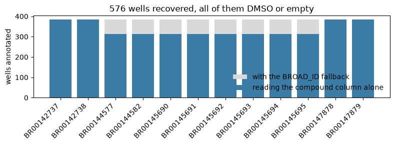
Eight plates lose 72 wells each that way, 576 in all. Every one of them is a control or a deliberately empty well, which is exactly the set you cannot afford to drop.

The design, as the plate sees it

The dosed plates are laid out as a dilution series across the plate, with vehicle and empty wells interleaved. Drawing the concentration on the well grid shows the design and where the controls sit:

dosed_plate = "BR00145690"
fig, axes = plt.subplots(1, 2, figsize=(11, 3.4))
mt.pl.plate(adata, color="Metadata_Concentration", plate=dosed_plate, ax=axes[0], cmap="magma")
axes[0].set_title(f"{dosed_plate}: concentration (µM)")
mt.pl.plate(adata, color="Metadata_CellCount", plate=dosed_plate, ax=axes[1], cmap="viridis")
axes[1].set_title(f"{dosed_plate}: cells per well")
fig.tight_layout()

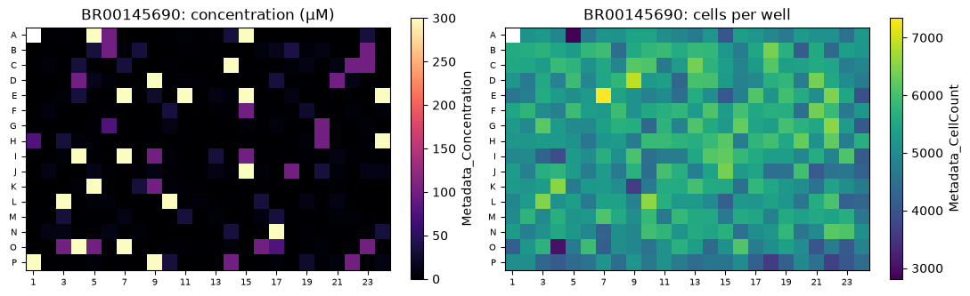
The blank cells on the left are the wells with no concentration to show: DMSO and the empties. On the right the same plate in cell counts, which is where a dose series first becomes visible — the columns that carry the highest concentrations of the more toxic compounds are the sparsest.

Dose coverage

Concentrations are micromolar and span nearly six orders of magnitude. What matters for a curve fit is not the range but how many distinct concentrations each compound actually carries:

treated = obs[~obs["Metadata_Control"] & (obs["Metadata_Compound"].astype(str) != "EMPTY")]
doses = treated.groupby(["Metadata_CellLine", "Metadata_Compound"], observed=True)["Metadata_Concentration"].nunique()

fig, axes = plt.subplots(1, 2, figsize=(11, 3.2))
axes[0].hist(doses.to_numpy(), bins=np.arange(0.5, 12.5), color="#3a7ca5")
axes[0].axvline(5.5, color="#a93a31", ls="--", lw=1)
axes[0].set(
    xlabel="distinct concentrations",
    ylabel="compound and cell line pairs",
    title="four or fewer points cannot hold a 4PL",
)
for line, colour in (("U2OS", "#3a7ca5"), ("HepaRG", "#c1666b")):
    values = treated.loc[treated["Metadata_CellLine"] == line, "Metadata_Concentration"]
    axes[1].hist(np.log10(values[values > 0]), bins=40, alpha=0.6, color=colour, label=line)
axes[1].set(xlabel="log10 concentration (µM)", ylabel="wells", title="concentrations tested")
axes[1].legend(frameon=False)
fig.tight_layout()
print(f"{int((doses >= 6).sum())} compound-and-line pairs carry six or more concentrations")

56 compound-and-line pairs carry six or more concentrations

One concentration, written two ways

Two of the twelve plate maps record the dose to three decimals where the rest use four, so a single concentration arrives as both 3.704 and 3.7037. Nothing downstream can tell that these are one level: groupby splits a treatment’s wells across the two spellings, and dose_response() reports more distinct doses than were ever plated.

Metadata_Concentration keeps what each plate map recorded. Metadata_ConcentrationNominal is derived from it in the loader: levels that agree to within 1% are one level, named by the value the most wells carry, so every dose it holds is one that was actually written down rather than an average of two. It names Metadata_Perturbation, so replicates of a treatment stay in one group.

raw = obs["Metadata_Concentration"].to_numpy(dtype=float)
aligned = obs["Metadata_ConcentrationNominal"].to_numpy(dtype=float)
dosed = np.isfinite(raw) & (raw > 0)

print(f"distinct doses: {len(np.unique(raw[dosed]))} recorded, {len(np.unique(aligned[dosed]))} after aligning")
print(f"largest correction: {100 * np.max(np.abs(aligned[dosed] / raw[dosed] - 1)):.2f}%")
moved = pd.DataFrame({"recorded": raw[dosed], "aligned": aligned[dosed]}).query("recorded != aligned")
print(f"{len(moved)} of {int(dosed.sum())} dosed wells move")
moved.drop_duplicates().sort_values("aligned").head()

distinct doses: 141 recorded, 67 after aligning
largest correction: 0.88%
992 of 3880 dosed wells move

	recorded	aligned
3568	0.017	0.0171
3404	0.031	0.0309
3418	0.034	0.0343
3281	0.046	0.0457
3471	0.051	0.0514

What a dose series looks like in the cells

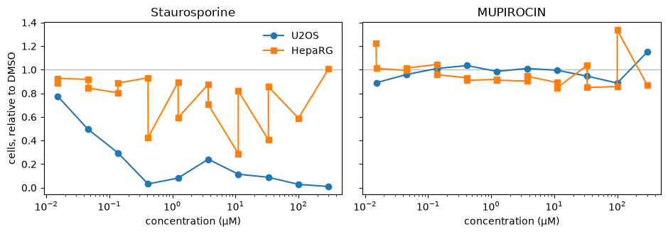
A dose series shows up first in the cell count. Staurosporine is a pan-kinase inhibitor and kills cells at concentrations where most compounds do nothing; mupirocin inhibits a bacterial enzyme and has no target in a human cell at all. They bracket what this plate map can show.

def per_dose(compound, line, column):
    """The median of `column` at each concentration of one compound in one cell line."""
    block = treated[(treated["Metadata_Compound"].astype(str) == compound) & (treated["Metadata_CellLine"] == line)]
    return block.groupby("Metadata_Concentration", observed=True)[column].median()


fig, axes = plt.subplots(1, 2, figsize=(9.5, 3.4), sharey=True)
for ax, compound in zip(axes, ["Staurosporine", "MUPIROCIN"], strict=False):
    for line, marker in (("U2OS", "o"), ("HepaRG", "s")):
        counts = per_dose(compound, line, "Metadata_CellCount")
        vehicle = obs[(obs["Metadata_CellLine"] == line) & obs["Metadata_Control"]]["Metadata_CellCount"].median()
        ax.plot(counts.index, counts.to_numpy() / vehicle, marker=marker, label=line)
    ax.set(xscale="log", xlabel="concentration (µM)", title=compound)
    ax.axhline(1.0, color="0.7", lw=0.8, zorder=0)
axes[0].set_ylabel("cells, relative to DMSO")
axes[0].legend(frameon=False)
fig.tight_layout()

What it is for

The count is only the crudest readout. A compound can reshape cells long before it kills any, and a concentration-response fit on the profile finds that earlier than a fit on the count does. 11. Concentration response runs that analysis on this screen: the continuous hit call, what it does with compounds that never plateau, how to read it beside a cell count, and whether a call made in HepaRG survives in U2OS.

One property of the design belongs here rather than there. This plate map spends its wells on concentrations rather than replicates, so a compound at one concentration usually sits in one or two wells. A per-concentration test is therefore thin, and the evidence lives in the shape across the whole series. That is what the dataset is for, and what it is not for.

Caveats

• The profiles arrive normalized and feature-selected per batch, so the two cell lines were processed apart. Compare distances within a line; across lines, compare calls.

• HepaRG has eight plates and U2OS two. The HepaRG calls rest on more wells.

• The assay development batch doses DMSO itself, so a control well there carries a concentration. Metadata_Control marks the compound, not the dose.

• EMPTY wells hold no compound and no vehicle. They keep their label rather than being dropped, and should be excluded before scoring, as above.

• Concentrations are micromolar throughout, including the assay development batch, which reports its own concentration_uM.