JUMP-Target-2

One 384-well plate map of 302 compounds, DMSO among them, that every JUMP laboratory ran [Chandrasekaran et al., 2023]. Differences between plates from different sources are therefore technical, which is what this dataset is for. All 141 plates are pinned, from eleven sources and 107 batches. source_9 ran the map four times over on 1536-well plates, the others on 384-well plates.

import mantispy as mt

adata = mt.ds.jump_target2()
adata

AnnData object with n_obs × n_vars = 5374 × 3634
    obs: 'Metadata_Source', 'Metadata_Plate', 'Metadata_Well', 'Metadata_CellCount', 'Metadata_SiteCount', 'Metadata_JCP2022', 'Metadata_InChIKey', 'Metadata_Perturbation', 'Metadata_Control', 'Metadata_Batch'
    var: 'object', 'feature_group', 'feature', 'channel', 'scale', 'angle', 'gray_levels', 'radial_bin', 'params', 'is_feature'
    uns: 'mantispy'
    layers: None (.X)

jump_target2() loads one plate from each source, unless plates= names others or plates=None asks for all 141.

Source

file	from	holds
<plate>.parquet	Cell Painting Gallery, cpg0016-jump/<source>/workspace/profiles	the well-level profiles, with source, plate and well
<plate>.csv	Cell Painting Gallery, cpg0016-jump/<source>/workspace/backend	pycytominer’s aggregate of the same plate, which carries the counts
plate.csv.gz, well.csv.gz, compound.csv.gz	jump-cellpainting/datasets	what each well received

The backend table is 33 to 57 MB per plate for two columns of it, and will be rehosted as part of this dataset’s h5ad.

Columns mantispy adds

column	how
Metadata_Batch	the batch directory the plate is filed under
Metadata_JCP2022, Metadata_InChIKey	well.csv.gz joined on source, plate and well, then compound.csv.gz
Metadata_Perturbation	Metadata_JCP2022
Metadata_Control	JCP2022_033924, DMSO
Metadata_CellCount	the backend table’s Metadata_Count_Cells, or its Metadata_Object_Count where it has no other
Metadata_SiteCount	the backend table’s Metadata_Site_Count

source_6’s backend tables publish Metadata_Object_Count and no Metadata_Count_Cells. On plate 110000294936 it matches the count jump-profiling-recipe uses in all 384 wells.

obs = adata.obs
obs.groupby(["Metadata_Source", "Metadata_Batch", "Metadata_Plate"], observed=True).agg(
    wells=("Metadata_Well", "size"),
    DMSO=("Metadata_Control", "sum"),
    median_cells=("Metadata_CellCount", "median"),
)

			wells	DMSO	median_cells
Metadata_Source	Metadata_Batch	Metadata_Plate
source_10	2021_08_03_U2OS_48_hr_run12	Dest210726-160150	384	64	745.5
source_11	Batch2	LM37-70_1	383	64	2026.0
source_13	20220914_Run1	CP-CC9-R1-29	384	64	3291.0
source_2	20210614_Batch_1	1053600674	383	65	1984.0
source_3	CP59	JCPQC051	384	64	1432.5
source_4	2021_04_26_Batch1	BR00121438	384	64	1268.0
source_5	JUMPCPE-20210623-Run02_20210624_225846	ACPJUM012	384	64	2144.0
source_6	p210914CPU2OS48hw384exp027JUMP	110000294936	384	65	1885.5
source_7	20210719_Run1	CP1-SC1-25	384	64	2585.0
source_8	J1	A1170384	384	64	1628.0
source_9	20210825_Run6	GR00003394	1536	256	1287.0

Fields of view

Metadata_Site_Count counts the fields of view that contributed cells, not those imaged. The sources image different numbers: four a well at source_9, six at source_10, twelve at source_2 and nine elsewhere. Most wells below their plate’s number are nearly empty, but not all of them:

# The fields each plate imaged.
imaged = obs.groupby("Metadata_Plate", observed=True)["Metadata_SiteCount"].transform("median")
short = obs[obs["Metadata_SiteCount"] < imaged]
print(
    f"{len(short)} of {adata.n_obs} wells, {int((short['Metadata_CellCount'] <= 50).sum())} of them with 50 cells or fewer"
)
columns = ["Metadata_Plate", "Metadata_Well", "Metadata_SiteCount", "Metadata_CellCount"]
short.sort_values("Metadata_CellCount", ascending=False)[columns].head(6)

27 of 5374 wells, 24 of them with 50 cells or fewer

	Metadata_Plate	Metadata_Well	Metadata_SiteCount	Metadata_CellCount
1191	ACPJUM012	B17	8.0	1751.0
1807	110000294936	L09	8.0	193.0
2458	A1170384	G12	8.0	61.0
4840	LM37-70_1	J19	8.0	27.0
1019	BR00121438	K13	8.0	26.0
920	BR00121438	G10	8.0	23.0

B17 on ACPJUM012 lost a field outright with 1,751 cells, while L09 on 110000294936 left one empty with 193. Either way, the count covers eight fields where the plate’s other wells cover nine, which is why cytotoxicity() compares cells per field. The one well above its plate’s number, P09 on CP-CC9-R1-29, reports 18 fields and 6,134 cells: twice its plate’s median well, and the same per field, as if it were imaged twice.

What it looks like

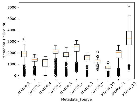
The sources seed different numbers of cells, more than fourfold apart from source_10 to source_13. Within a plate, the strongest compounds are cytotoxic.

ax = mt.pl.cell_counts(adata, groupby="Metadata_Source")

axes = mt.pl.plate(adata, color="Metadata_CellCount", groupby="Metadata_Source")

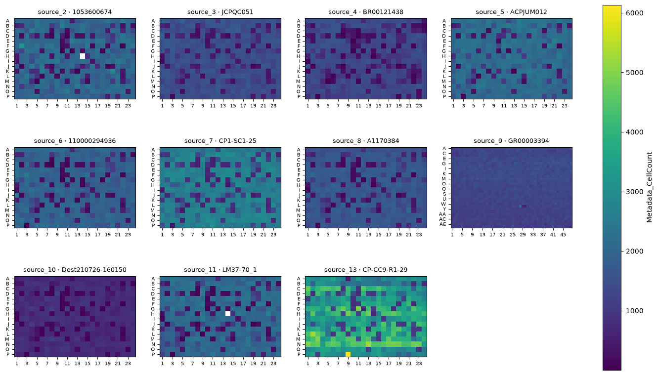
On one scale, the same wells are dark on every 384-well plate, because every source ran the same map: 55 wells hold less than half their plate’s median count on at least eight of the ten.

ax = mt.pl.plate(adata, color="Metadata_CellCount", plate="BR00121438")

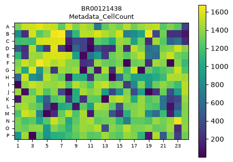
Wells with a fraction of the plate’s cells are why a distance from the controls alone ranks cell death as the strongest phenotype on this plate; cytotoxicity() flags them.